
Abstraction by Interchangeability in Resource Allocation
Proceedings of the Fourteenth International Joint Conference on Artificial Intelligence. Planning. Pages 1694-1702.
© 1995 International Joint Conferences on Artificial Intelligence
Abstract
Resource allocation is a difficult constraint satisfaction problem that has many practical applications. Fully automatic systems are often rejected by the ultimate users because, in many real-world environments, constraints cannot be formalized completely. On the other hand, humans are overwhelmed by the complexity of their task. We present a new way of solving the resource allocation, where a computer builds dynamic abstractions that simplify problem solving to the point that the user can intervene in the solution of the problem. These abstractions are based on the concept of interchangeability introduced by Freuder. In this paper, we describe a heuristic for decomposing a resource allocation problem into abstractions that reflect interchangeable sets of tasks or resources. We assess the "quality" of the discovered neighborhood interchangeable sets by comparing them to the ones obtained by the exact algorithm described by Freuder, both for data taken from a real-world application and for randomly generated problems.
- Esther Arkin and Ellen Silverberg. Scheduling Jobs with Fixed Start and End Times. Discrete Applied Mathematics, 18:1-8, 1987.
- Brent W. Benson and Eugene C. Freuder. Inter- changeability Preprocessing Can Improve Forward Checking Search. In Proc. of the 10th EGA!, pages 28-30, Vienna, Austria, 1992.
- Berthe Y. Choueiry. Abstraction Methods for Re- source Allocation. PhD thesis, Swiss Federal Institute ofTechnolody in Lausanne (EPFL), Switzerland, Oc- tober 1994. Thesis No 1292.
- Berthe Y. Choueiry and Boi Faltings. A Decompo- sition Heuristic for Resource Allocation. In Proc. of the 11 th EGA!, pages 585-589, Amsterdam, The Netherlands, 1994.
- Eugene C. Freuder. Eliminating Interchangeable Val- ues in Constraint Satisfaction Problems. In Proc. of AAAI-91, pages 227-233, Anaheim, CA, 1991.
- Nancy B. Lehrer. Knowledge Representation Speci- fication Language {KRSL). DARPA/Rome Labora-- tory Planning and Scheduling Initiative, June 1992. DRAFT.
- Alan K. Mackworth. Consistency in Networks of Re- lations. Artificial Intelligence, 8:99-118, 1977.
- Edward R. Scheinerman. An Evolution of Interval Graphs. Discrete Mathematics, 82:287-302, 1990.
References were extracted automatically from the PDF and may contain errors.
Full text extracted automatically from the PDF; figures, tables and equations may differ. The PDF is the version of record.
1 Introduction and motivation
The resource allocation (RA) problem is to assign re sources to a set of tasks, scheduled at given time inter vals, such that no resource is assigned to two different tasks at the same time. It arises in many real-world applications.
- In manufacturing, once the various jobs have been scheduled, it appears as the problem of distribut ing tools to the machining centers and of allocating routing vehicles to transfer the material.
- In the operating units of a hospital, the availability of personnel and the program of surgical operations to be executed are decided at various administrative levels, days or weeks in advance. On a daily basis, one or two human operators distribute the qualified personnel (nurses and technicians) to the surgical operations as required.
- In an airline company, the problem arises for al locating, to the various scheduled flights, aircraft,
cabin crew, gates; as well as personnel, vehicles, and equipment for catering, baggage handling, cleaning, and fuel refilling.
Fig. 1 shows an example of a resource allocation prob lem. The problem can be represented as interval orders, as shown on the left of Fig. 1. In this paper, however,
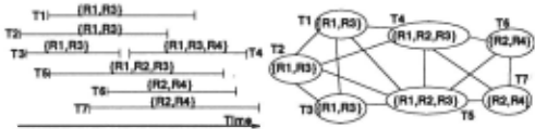
Figure 1: Left: Interval orders: a schedule of seven tasks whose start time and duration are fixed. For each task, a set of possible resources is shown. Right: the corresponding constraint graph.
we model the resource allocation problem as a discrete Constraint Satisfaction Problem (CSP) [7] in which the constraints among variables are binary and denote mu tual exclusion with respect to the values, as shown in Fig. 1 right. The nodes of the constraint graph repre sent tasks to be executed, and their labels are sets of resources that can carry out the tasks. Arcs link nodes that intersect in time and have at least one resource in common. Note that we consider only resources that are reusable and non-sharable, see [6].
Complexity. Arkin and Silverberg [1] showed that the resource allocation problem is NP-complete (i.e., the existence of a polynomial solution method is unlikely). In [3], we showed that an optimization version of the resource allocation problem in which certain tasks (com pulsory tasks) must absolutely be allocated a resource and the number of the remaining ones (optional tasks) must be maximized is at least as difficult as MAXSNP complete, for which the existence of a polynomial-time approximation scheme is unlikely.
Requirement: interactivity vs. automation. Of ten, constraints cannot be exhaustively enumerated. For example, the constraint that two persons do not work well together is often not formalized. Moreover, con straints may vary over time. For example, a person may be sick and unable to carry out certain tasks. Fully au tomatic methods are, therefore, often rejected by the ultimate users, who have to revise solutions with the full complexity of the original problem. Thus, it is impor tant to present them with compact representations that simplify the problem.
Abstractions as a new perspective. In this paper, we investigate the use of computers to dynamically build abstractions that structure the problem space and al low the users to solve the problem interactively. In [4], we introduced a heuristic called the Value-Assignment Delay heuristic (VAD) for decomposing a resource al location problem into sub-problems. The VAD tries to solve sub-problems independently and isolates con flicts between them. The tradeoffs of using this decom position scheme and a comparison to related work in the scheduling and CSP literature are reported in [3; 4].
By decomposing a problem, the VAD implicitly gener ates equivalence classes of resources and tasks. We argue that these new objects structure the solution space of a resource allocation problem in a compact manner and identify equivalent choices. Thus, they serve as a basis for abstraction. In this paper, we identify these vari ous abstraction classes and characterize them in terms of interchangeability sets [5].
The paper is organized as follows. In Section 2, we recall the main definitions of interchangeability that are of interest to us. In Section 3, we describe and formalize the interchangeable sets discovered by the VAD; then we show how they can be used as abstractions to simplify problem solving. In Section 4, we evaluate the discovered neighborhood interchangeable sets with respect to the ones found by the exact algorithm. Section 5 presents our conclusions.
2 Interchangeability: definitions
In [5], Freuder introduces the concept of interchangeabil ity and defines various kinds of value interchangeability. In this section, we quickly recall the definitions of inter est to us. The phrase "(i,j) satisfies C" means that values i and j for two variables linked by a constraint C are consistent with respect to this constraint.
Definition 1 Full interchangeability: A value b for a CSP variable V is fully interchangeable with a value c for V if and only if every solution to the CSP that assigns b to V remains a solution when cis substituted for b in V and vice versa.
This means that values band c can be switched for vari able V in a given solution without affecting at all the rest of the problem and regardless of the constraints that apply to the variables. Freuder notices that computing fully interchangeable sets may require, in general, com puting all solutions, which can be a quite costly opera tion.
Definition 2 Neighborhood interchangeability: A value b for a CSP variable V is neighborhood interchangeable with a value c for V if and only if for every constraint C
on V:
Neighborhood interchangeability is a stronger condi tion than full interchangeability (i.e., not all fully inter changeable sets are neighborhood interchangeable), but is easier to compute. Freuder describes a polynomial time procedure for computing all neighborhood inter changeable sets 1 .
Definition 3 Substitutability: Given two values b and c for a CSP variable V, b is substitutable for c if and only if substituting b in any solution involving c yields another solution.
Substitutability is 'one-way' full interchangeability.
Definition 4 Neighborhood substitutability: For two values b and c, for a CSP variable V, b is neighborhood substitutable for c if and only if for every constraint C on V:
Neighborhood substitutability is 'one-way' neighbor hood interchangeability.
Definition 5 Partial Interchangeability: Two values are partially interchangeable with respect to a subset S of variables if and only if any solution involving one implies a solution involving the other, with possibly dif ferent values for variables in S.
Note that full interchangeability is partial interchange ability with S = 0. Indeed, Freuder outlines that: "Par tial interchangeability captures the idea that values for variables may differ among themselves, but be fully in terchangeable with respect to the world".
Using partial interchangeability, we may isolate a sub problem in which the partial solution can be affected by a change of the value of a variable in the isolated sub-problem, without having to update the rest of the solution. This idea of localizing the effect of a modifica tion is very important in scheduling applications, where one tries to keep the stability of a global solution while adjusting a partial solution locally to accommodate un foreseen events. Thus, partial interchangeability sets can serve as a basis for reactive scheduling strategies. In [5], Freuder argues that interchangeable values are redun dant and their removal simplifies the problem space.
3 Interchangeability in RA
The algorithm described in [5] is applicable to all types of constraints, however, it only finds neighborhood inter changeabilities (NI) 2 · Below, we introduce a decomposi tion heuristic, called the VAD heuristic, which is only applicable to constraints of mutual exclusion; but, in addition to the NI sets, it also determines other types of interchangeability for which no other algorithm is known so far.
1 The worst-case complexity of this procedure is O(n 2 a 2 ), where n is the number of nodes and a is the domain size.
2 In [5], Freuder proposes also a generalized version for finding k-interchangeability.
3.1 The Value-Assignment Delay heuristic
The idea of the VAD heuristic, as stated in [4], is as fol lows: "Delay the assignment of the most solicited values in a list coloring problem and try to solve the simplified problem without them. Distribute the delayed values to those variables that really cannot do without them."
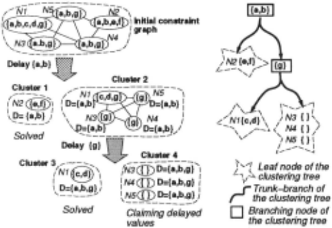
The application of this heuristic to a simple example is shown in Fig. 2. In the first step, the assignment of values a and b is delayed. The set {a, b} is called the set of delayed values. This has the effect of breaking up the initial graph into two components, because N2 now has no value in common with, and thus no link to, the rest of the graph. This process is repeated itera tively, and yields a clustering tree in which the leaves represent simplified sub-problems, the nodes are sets of delayed values and the branches show how these com ponents relate (Fig. 2 right). Some of the sub-problems can be easily solved in isolation without any effect on the rest of the problem. For example, nodes in Cluster1 and Cluster3 can be assigned any element in { e,!} and { c, d} respectively. Such commitments are safe and never need to be undone. All the other parts need to claim de-
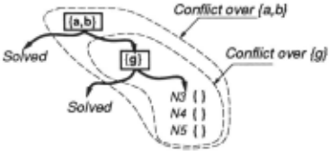
layed resources for their solution. A conflict is defined around each value set claimed by several nodes in the leaves, see Fig 3. Conflicts may be resolved according to some heuristic and domain dependent preferences or by interactive users' intervention. Users may decide to relax constraints and "borrow" any of the values that remain unassigned.
By isolating easy sub-problems, identifying conflicts, and localizing interactions among the various compo nents of a resource allocation problem, the heuristic defines a tree structure useful for interactive decision making. The algorithm and termination criteria are de scribed in detail in [4; 3], where we show that the worst case complexity of the method is O(n 3 +(n+a)an1oga), n being the number of tasks and a the number of re sources.
3.2 Interchangeability found by the VAD
The VAD heuristic is by itself an abstraction technique. By grouping values on the trunk of the partitioning tree and by pushing variables into the leaves, it implicitly cre ates aggregates of similar tasks and resources: it makes explicit the similarities and differences among these enti ties as far as value contention is concerned. For instance, for the example shown in Fig. 2, the VAD discovered that c and d are equivalent with respect to N1 and that a and b are equivalent with respect to N1, N2, ... , Ns.
Thus, the VAD heuristic implicitly builds pools of resources and aggregates of tasks, which are equiva lence classes of objects or objects that are interchange able with respect to the constraints. These equivalence classes can be considered as problem-specific abstrac tions useful for solving this particular problem instance. We now show how the components discovered by the VAD identify interchangeable sets.
We use a simple example 3 taken from real-life case study to illustrate the various kinds of interchangeability discovered during decomposition by the VAD heuristic. The problem domain is the allocation of operating rooms and technicians to surgical operations in a hospital.
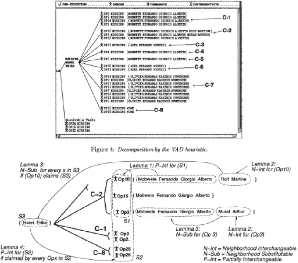
In Fig. 4 right, we show the tree structure generated by the application of the VAD heuristic and the resources delayed at the branching nodes. For each leaf cluster, we display the tasks (surgical operations) but not the links between the tasks as in a constraint graph. The proposition ":1: Op:z: missing" indicates that Op:z: needs to be allocated a resource of type gar~on. The set of re sources following the proposition is the set of values that have not been delayed and are still directly available. In this example, the set {Henri, Erika} was delayed and the initial problem broke down into eight leaves.
Fig. 5 shows the interchangeability relations dis covered in one of the leaf clusters of Fig. 4. For a variable Vi in a leaf cluster, {vi} denotes the set of values still available for \ti. For instance, for variable Op10 in cluster C2 in Fig. 4, {vi} = {Mobwete, Fernando, Giorgio, Alberto, Rolf, Martine}. We claim that:
Lemma 1 For every variable Vi in a leaf cluster C, all values in the set n { Vj} are partially interchangeable V;EC
with respect to S = {Vj E C}.
3 This is the example "testl-a" of Table 1 in Section 4, slightly modified to illustrate all the types of interchange ability addressed in this section.
rt ~--IJIECOI711f ..··· ·· · · ·· *-.... .. ..... (n~ .. ·..: . . ... .. XJii5liiiMNTI~~;.:.:..;;: .
Proof: Let T = n {vi}. Since the values in T have V;EC
not been delayed, they are needed by no other variable in the problem within the time window of the cluster C, except the ones in C. Thus, no conflict with variables outside Cis possible and any decision about the assign ment of elements ofT can only affect variables in C. Since any value in T is acceptable for any variable in the cluster, two values for a variable can be always swapped in any solution by a permutation of the values in T over the variables in C, for instance. Thus, there cannot be solutions involving one value in T without there being solutions involving the other values in T. D
Example from Fig. 5: In C-2, {Mobwete, Fernando, Giorgio, Alberto} are partially interchangeable for {Op10 , 0Pt5. Op3 }.
For lemmas 2 and 3, let Ui denote the set of values uniquely available to variable Vi in cluster c. ui is given by the formula ui ={vi}- u {vj}· V; EC,j f. i
Lemma 2 For every variable V; in a leaf cluster C , all values in the set ui are neighborhood interchangeable.
Proof: Ui may not create any conflict outside C for the same reason as in the proof of Lemma 1. Within C, all values in ui are possible only for Vi, by construction. Thus no conflict is possible with any other variable {Vj E C,j=f=i}. D
Example from Fig. 5: In C-2, {Rolf, Martine} are neighborhood interchangeable for Op10 , and {Murat, Arthur} are neighborhood interchangeable for Op3·
Lemma 3 For every variable Vi in a leaf cluster C, each value in Ui is neighborhood substitutable for every other value in the label of \ti. In particular, each value in Ui is neighborhood substitutable for every value in n { Vj} V;EG
and for every value in every delayed set that Vi may claim.
Proof: Since no value in Ui was delayed, this means that Ui is needed only for Vi during Vi and assigning any element of Ui to Vi does not rule out any choice for the rest of the problem. Therefore, the set of values for nodes adjacent to Vi, for the case where Vi is assigned an element of Ui, will be a superset of that for the case where it is assigned any other value in its label. D
Example from Fig. 5: In C-2, each of {Rolf, Martine} are neighborhood substitutable for each of {Henri, Erika, Mobwete, Fernando, Giorgio, Alberto} for Opw.
Lemma 4 All values in a given set of delayed values D are partially interchangeable with respect to the setS of variables located downstream that claim D.
Proof: The set of delayed values is chosen at each step as the set of values simultaneously claimed by a set of variables, see [4]. Thus, if a variable claims any element of the set of delayed values, it also claims all the others, by construction. D
Example from Figures 4 and 5: {Henri, Erika} are partially interchangeable for all the nodes in the leaf clusters Ct. ... , C8 since they are admissible for all these nodes (although this information is not explicitly shown).
In [5], Freuder suggests that interchangeability can also be computed dynamically during problem resolu tion, (i.e., dynamic interchangeability). An example of this is shown in Fig. 6. Suppose that a conflict resolution procedure (or the user), decides to assign b to Task K. The delayed value set {a} is now fully interchangeable with { e, f} for variable Task L.
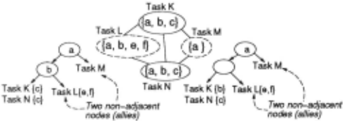
Lemma 5 Any delayed value claimed only by a set N of non-adjacent nodes 4 is fully interchangeable with all {vi} for each Vi E N.
4 Two non-adjacent variables are called allies since, when
Proof: Since the values in the delayed set are claimed only by non-adjacent nodes, whether they are assigned to two or more nodes simultaneously cannot affect the prob lem in any way. In particular, each of them is neighbor hood substitutable for all {vi} in each \ti. Since all {vi} can be proven neighborhood substitutable for each of these values using Lemma 3, they are fully interchang~ able. D
As these lemmas show, in addition to the NI sets, the VAD also determines other types of interchangeability for which no other algorithm is known so far. In the case of partial interchangeability, the VAD also determines the sets of nodes with respect to which the values are interchangeable.
3.3 Interchangeable sets as abstractions
We claim that the VAD decomposition scheme structures the solution space into compact families of partial solu tions: qualitatively equivalent solutions can be generated by locally modifying the partial solutions in the isolated interchangeable sets. In Fig. 4, it is easy to see that many solutions can be generated simply by switching partially interchangeable values for tasks in the same leaf clus ter. This switching operation affects only the nodes in the leaf, while keeping the rest of the 'world' unchanged. Thus, by only viewing the clustering tree generated by the VAD, the user can easily assess the variety of pos sible solutions. Classical enumerative methods fail to organize the solution space in such a compact manner: they present solutions to the users in a jumble without showing similarities and differences between alternative solutions. In particular, they fail to identify the bound aries within which the effect of a change remains local.
In interactive problem solving, interchangeable sets help the human decision maker to view alternative choices in a concise way. Full or neighborhood inter changeable values can be replaced by one 'meta-value'. Partial interchangeability identifies the boundaries in which changes are permitted. When a value a is neigh borhood substitutable for a value b for a given variable the user is guaranteed to be able to replace b by a any time a solution involving b for the variable is found, if b is not acceptable for some unquantifiable or subjective reason.
In search, the main advantages of discovering inter changeability sets are: (1) compacting the solution space representation by grouping families of solutions that are equivalent, thus allowing the search process to remain as local as possible, and (2) enhancing the performance of backtracking and consistency checking by removing redundant values.
In dynamic concept formation, see [3], interchang~ ability identifies groups of objects (sets of variables and sets of values) to become the basic components for a generalization process aimed at providing explanation.
4 Evaluation of NI sets
The VAD heuristic is not guaranteed to discover all inter changeable sets. Its performance depends on the structure of the problem at hand. The interchangeable sets approximated by the VAD may differ from the exact ones in two ways: (1) the sets discovered by the VAD may be only subsets of the largest possible ones and (2) some possible sets may be missed.
they claim the same delayed set, they may be assigned values from this set simultaneously, see [4].
The conditions under which the VAD discovers all ex act sets of interchangeable values are so far unknown. We have evaluated the performance both on data from a case study in a hospital and on a variety of randomly generated resource allocation problems. The character istics of the hospital case-study in terms of CSP mea sures are reported in Table 1. The random problems are generated following on the evolutionary model for gen erating random interval orders by Scheinerman [8] and a resource model where the number and selection of re- sources follow a uniform distribution.
We report the results only for problem sizes n = 20 and n = 50, while varying the adjacency probability 5 of the interval graph in {0.1, 0.2, ... , 0.9, 0.99}, and th · d · · {n 2n 9n } D e maximum omam Size a = 10 , 10 , ... , lQ, n . ror each case, ten random problems were generated and each point in the experiments reported below is obtained by taking the average over the ten cases.
Each time, we have compared the NI sets obtained by the VAD decomposition with those obtained by the exact algorithm by Freuder according to the two criteria introduced above (i.e., maximality and existence).
Let G = (V, E) be a constraint graph of V vertices (or variables) and E edges (or constraints), and
- se(v) be the set of NI values for variable v found by the exact algorithm by Freuder [5]
- Statal= {se(v);'v'v E V and se(v) #- 0} be the set of all NI sets for the variables
- s11 ( v) be the set of NI values for variable v identified by our decomposition method, s11 (v) ~ se(v)
- Vmissed = {v; Sv(v) c se(v)}, this is the set of variables with non empty NI sets and for which the NI sets discovered by the VAD are different from the exact ones
- V1 = {v E V; se(v) #- 0}, this is the set of variables that have a non empty NI set.
We now consider the results of the evaluation regard ing three different criteria: occurrence Pt (1), coverage P2 (2), and accuracy P3 (3) 6 as discussed below.
Occurrence: existence of NI sets. p1 measures the "occurrence" of neighborhood interchangeability in a problem and is computed using the exact algorithm. A small value for Pt indicates that few NI sets exist in G.
In the real-world examples reported in Table 1, we no tice that the occurrence of NI is rather rare (Pt is small).
5 The adjacency probability, also called constraint proba bility, is p = ~.where e is the number of edges.
6 Existence ~rNI sets is measured by Pt and maximality by P2 and P3·
In fact, the other types of interchangeability character ized in Section 3.2 seem to occur more often (for exam ple, see Fig. 5). The evaluation of the latter has not yet been carried out.
For the randomly generated data, Fig. 7 shows the followin~ behavior: (1) As Benson and Freuder experi enced [2J, only problems of small adjacency probability present interchangeability features: the number of NI sets becomes nearly zero for p > 0.4. (2) For problems with a "small" value for p, the number of interchange- able sets increases with the number of resources. (3) The number of interchangeable sets decreases with the size of the problem 7 even when the ratio of the number of val ues to the number of variables ( ~) is held constant. This is foreseeable because the resources are not structured (chaos increases).
Coverage: how many NI sets are approximated. p2 measures the number of sets that are affected by the behavior of the VAD. A small value for P2 indicates that few of the NI sets discovered by the VAD are different from the exact ones. A large value for p2 means that many sets are truncated.
For the set ofreal-world data described in Table 1, no set of neighborhood interchangeable values was missed (p2 = 0 in all cases). For the randomly generated problems, the measured values of P2 are reported in Fig. 8 and Table 2. We can draw the following observations from Fig. 8. For problems with small values for p, very few NI sets are truncated. The VAD nearly finds all exact sets. This is the most important region since it contains most NI sets (p1 is large). When p increases, the number of NI sets that are not complete also increases. However, one should bear in mind that, for these problems, Pt is small, which means that few NI sets exist. This explains why p2 deteriorates significantly even though the proportion of NI sets found is still fairly high.
Accuracy: the extent of NI sets approximation. The parameter p3 measures the accuracy to which the VAD computes the NI sets 8
A small value for p3 indicates those sets affected by the approximation are heavily distorted (truncated). A value p3 = 0 means that all NI sets were completely missed by the VAD. Large values for P3 are desirable since they indicate that the NI sets discovered by the VAD are hardly altered.
For the set of real-world data described in Table 1, all the discovered NI sets were exact (p3 is undefined in all cases).
7 The number of NI was so small (too small for any eval uation) for the cases n = 50 and a::::; 50 that we decided to generate also, for this problem size, the cases a = 60, 70, and
80. 8 Note that P3 is defined only when \t;,..i .. ed -10.
| CSP parameterS T Evaluation of NI | ||
|---|---|---|
| II I test- id | n a d t T | sets rit i>2 P3 |
| II testl-a | 22 5 0.376 0.094 0.136 | 0 - |
| test2 | 25 6 0.529 0.108 | 0 - |
| test3 | 0.04 25 5 0.41 0.137 0.04 | - |
| test4 | 35 7 0.405 0.093 | 0 0 - - |
| test5 | 36 8 0.455 0.087 | - |
| test1-b | 0 44 24 0.420 0.043 0 | - - - |
| test6-a. | 47 25 0.570 0.043 | 0 - - |
| test -a. | 49 26 0.454 0.041 | - |
| test1 | 66 24 0.433 0.037 | 0 - 0.046 0 - |
| testS | 68 28 0.43 .038 0.015 | 0 - |
| test9 | 72 29 0.444 0.037 | 0 - - |
The numerical results for the random problems are reported in Table 3 and should be understood in light of the previous ones, (i.e., Pl and P2): Pl percent of the variables have non empty NI sets; P2 percent of these sets are distorted by the VAD; and the distorted sets are p3 percent accurate. From comparing the results, one may conclude that:
- Problems with small adjacency probability (p is small) present many NI sets (Pl is large). Many of these NI sets are faithfully rendered by the VAD (p2 is small). Those that are approximated are not seri ously altered (p3 is large). For example, for p = 0.1, n = 20, a = 14, we have Pl = 26.0%, P2 = 7.4%, P3 = 56.0%.
- Conversely, problems with high adjacency probabil ity (pis big) present few NI sets (p1 is small) many of which are distorted by the VAD (p2 is large) and those that are approximated are seriously affected (p3 is small).
5 Conclusion
Because a changing and complex world cannot be com pletely formalized, resource allocation problems should not be addressed using fully automatic methods. In this paper, we propose the paradigm of dynamic abstractions as a new way of applying computers for such tasks. Here, a computer is used essentially to structure a problem space into relevant abstractions. This allows a user to participate in solving the actual problem while taking into account the unformalized constraints which hold at that moment.
We claim that interchangeability is a useful notion to characterize adequate abstractions, then we present and analyze a heuristic for dynamically generating abstrac tions for resource allocation. Although one still has to study the theoretical conditions under which the discov ered NI sets are maximally defined, the approximation of NI sets by the VAD is acceptable given that:
- NI sets are more frequent in problems with small p and the effect of the "distortion" due to the VAD decreases with p.
- The VAD can be computationally less expensive
than the exact algorithm 9 ·
- The computation of NI sets is not the purpose of the VAD, whose goal is to localize interactions and conflicts among sub-problems; these results are only a fortunate "side effect".
As a general comment, we recall again that neigh borhood interchangeability is not the only type of in terchangeability discovered by the VAD and that there exists, so far, no other algorithm for computing other types of interchangeability except for the obvious pro cess of computing all possible solutions. Note that the possibility of discovering interchangeable sets increases in structured domains with some semantics. Thus, var ious real-world problems, such as scheduling, configura- tion, and design, may benefit greatly from finding in terchangeability sets. Note also that the three proposed parameters, Pl, p2, and p3, can be exploited to measure quality of interchangeable sets in general.
In future work, we hope to extend our approach in two directions: exploiting interchangeability sets in rescheduling and building a generalized theory of ab straction in CSPs using interchangeability concepts.
Acknowledgments
The authors are indebted to Dean Allemang, Guevara Noubir, Bradley Richards and the anonymous reviewers for their comments.
@inproceedings{ijcai1995p218,
  title     = {Abstraction by Interchangeability in Resource Allocation},
  author    = {Choueiry, Berthe Y. and Faltings, Boi and Weigel, Rainer},
  booktitle = {Proceedings of the Fourteenth International Joint Conference on
               Artificial Intelligence, {IJCAI-95}},
  publisher = {International Joint Conferences on Artificial Intelligence},
  editor    = {Chris S. Mellish},
  pages     = {1694--1702},
  year      = {1995},
  note      = {Planning},
  url       = {https://ijcai.org/proceedings/1995/218},
}
TY - CPAPER TI - Abstraction by Interchangeability in Resource Allocation AU - Choueiry, Berthe Y. AU - Faltings, Boi AU - Weigel, Rainer T2 - Proceedings of the Fourteenth International Joint Conference on Artificial Intelligence, IJCAI-95 PB - International Joint Conferences on Artificial Intelligence PY - 1995 SP - 1694 EP - 1702 UR - https://ijcai.org/proceedings/1995/218 ER -Copied
Machine-readable versions of this paper, for tools and AI agents:





