
Computing Circumscription Revisited: Preliminary Report
Proceedings of the Fourteenth International Joint Conference on Artificial Intelligence. Non-monotonic Reasoning. Pages 1502-1507.
Abstract
We provide a general method which can be used in an algorithmic manner to reduce certain classes of 2nd-order circumscription axioms to logically equivalent 1st-order formulas. The algorithm takes as input an arbitrary 2nd-or~er formula and either returns as output an eqmvalent 1st-order formula, or terminates with failure. In addition to demonstrating the algorithm by applying it to various circumscriptive theories, we analyze its strength and provi~e formal subsumption results based on comparison with existing approaches.
- [Ackermann, 1935] W. Ackermann. Untersuchungen iiber das eliminationsproblem der mathematischen logik. Mathematische Annalen, 110:39o-413, 1935.
- [Ackermann, 1954] W. Ackermann. Solvable Cases of the Decision Problem. North-Holland, Amsterdam, 1954.
- [Benthem, 1983] J. Van Benthem. Modal Logic and Classical Logic. Bibliopolis, Napoli, 1983.
- [Benthem, 1984] J. Van Benthem. Correspondence the- ory. In D. Gabbay and F. Guenthner, editors, Hand- book of Philosophical Logic, volume 2, pages 167-247.
- D. Reidel Pub. Co., 1984.
- [Doherty et al., 1994] P. Doherty, W. Luk.aszewicz, and A. Szalas. Computing circumscription revisited: A reduction algorithm. Technical Report LiTH- IDA-R-94-42, Linkoping University, 1994. URL: http:/ fwww.ida.liu.seflabs/rkllabfpeoplefpatdo/. Link
- [Gabbay and Ohlbach, 1992] D. Gabbay and H. J. Ohlbach. Quantifier elimination in second-order pred- icate logic. Technical Report MPI-I-92-231, Max- Planck Institut fiir Informatik, 1992.
- [Gelfond and Lifschitz, 1989] M. Gelfond and V. Lifs- chitz. Compiling circumscriptive theories into logic programs. In Proc. 2nd Int'l Workshop on Non- Monotonic Reasoning, volume 346 of Lecture Notes in Artificial Intelligence, pages 74-99, 1989.
- [Ginsberg, 1989] M. L. Ginsberg. A circumscriptive the- orem prover. Artificial Intelligence, 39:209-230, 1989.
- [Kolaitis and Papadimitriou, 1988] P. Kolaitis and C. Papadimitriou. Some computational aspects of circumscription. In Proc. AAAI-88, St. Paul, MN, pages 465-469, 1988.
- [Lifschitz, 1985] V. Lifschitz. Computing circumscrip- tion. In Proc. 9th IJCAI, Los Angeles, CA , pages 121-127, 1985.
- [Lifschitz, 1988] V. Lifschitz. Pointwise circumscription. In M. Ginsberg, editor, Readings in Non-Monotonic Reasoning, pages 179-193.
- [Lifschitz, 1994] V. Lifschitz. Circumscription. In D. M. Gabbay, C. J. Hogger, and J. A. Robinson, editors, Handbook of Logic in Artificial Intelligence and Logic Programming, volume 3, pages 297-352. Clarendon Press, Oxford, 1994.
- [Przymusinski, 1991] T . Przymusinski. An algorithm to compute circumscription. Artificial Intelligence, 38:49-73, 1991.
- [Rabinov, 1989] A. Rabinov. A generalization of col- lapsible cases of circumscription. Artificial Intelli- gence, 38:111-117, 1989.
- [Szalas, 1993] A. Szalas. On the correspondence between modal and classical logic: an automated approach. Journal of Logic and Computation, pages 605-620, 1993.
References were extracted automatically from the PDF and may contain errors.
Full text extracted automatically from the PDF; figures, tables and equations may differ. The PDF is the version of record.
1 Introduction and Preliminaries
In recent years, a great deal of attention has been de voted to logics of "commonsense" reasoning. Among the candidates proposed, circumscription [Lifschitz, 1994), has been perceived as an elegant mathematical tech nique for modeling nonmonotonic reasoning, but diffi cult to apply in practice. Practical application of cir cumscription is made difficult due to two problems. The first concerns the difficulty in finding the proper circum scriptive policy for particular domains of interest. The second concerns the 2nd-order nature of circumscription axioms and the difficulty in finding proper substitutions of predicate expressions for predicate variables so the axioms can be used for making inferences. There have been a number of proposals for dealing with the second problem ranging from compiling circumscriptive theories into logic programs [Gelfond and Lifschitz, 1989), to de veloping specialized inference methods for such theories [Ginsberg, 1989; Przymusinski, 1991).
A third alternative is to focus on the more general problem of finding methods for reducing 2nd-order for mulas to logically equivalent 1st-order formulas, where possible. Although some progress has been made using this approach, the class of 2nd-order circumscription for mulas shown to be reducible is not as large as one might desire, the reduction methods proposed are somewhat isolated relative to each other and, most importantly, Witold Lukaszewiczt Andrzej Szalas t Institute of Informatics Warsaw University 00-913 Warsaw 59, Poland the existing reduction theorems generally lack algorithmic procedures for doing the reductions. .
*Supported by Swedish TFR grant 93-270.
tsupported in part by KBN grant 3 P406 019 06 and ESPRIT BRA No. 6156-DRUMS II.
In this article, we provide a general method wh1~h can be used in an algorithmic manner to reduce certam classes of 2nd-order circumscription axioms to logically equivalent 1st-order formulas. The algorithm takes as input an arbitrary 2nd-order formula and either r~turns as output an equivalent 1st-order formula, or termmates with failure. Of course, failure does not imply that there is no 1st-order equivalent for the input, only that the algorithm can not find one. The class of 2nd-order for mulas, and analogously the class of circumscriptive theo ries which can be reduced, provably subsumes those cov ered by existing results. The algorithm can be applied successfully to circumscriptive theories which may in clude mixed quantifiers (some involving Skolemization), variable constants, n-ary tuples of minimized and varied predicates, separable, separated and in some cases, non separated formulas, and formulas with n-ary predicate variables, among others. In addition to demonstrat~ng the algorithm by applying it to some of these theones, we analyze its strength and provide formal subsumption results based on comparison with existing approaches.
Due to page limitations and the technical complexity of both circumscription and the algorithm we propose, we will be forced to remain brief with preliminaries. Conse quently, we assume familiarity with the various types of circumscription and existing reduction results. In gen eral, we will refer to the original articles for the relevant theorems and results. In addition, we provide only an informal description of the algorithm, but one that is adequate and sufficiently detailed for following the ex amples provided. For a detailed description of the al gorithm and proofs of the subsumption results, we refer the reader to the technical report [Doherty et al., 1994).
1.1 Notation
An n-ary predicate expression is any expression of the form >.x. A(x), where x is a tuple of n individual vari ables and A(x) is any formula of first- or second-order classical logic. If U is an n-ary predicate expression of the form >.x. A(x) and a is a tuple of n terms, then U(a) stands for A(a). As usual, a predicate constant P is identified with the predicate expression >.x. P(x). Similarly, a predicate variable <} is identified with the predicate expression >.x. <}(x).
Truth values true and false are denoted by T and 1., respectively.
If U and V are predicate expressions of the same arity, then U :5 V stands for VX. U(x) :) V(x). If ff = (U1 , ... , Un) and V = (V1, . . . , Vn) are similar tu ples of predicate expressions, i.e. ui and Vi are of the same arity, 1 :5 i :5 n, then U :5 V is an abbreviation for /\~=1 [U, :5 Vi]. We write U = V for (U :5 V) 1\ (V :5 U), and U < V for (U :5 V) 1\ ·(V :5 U).
If A is a formula, if= (cr1, .. . , ern) and 8 =:. (81, ... , 8n) are tuples of any expressions, then A(u +-- 6) stands for the formula obtained from A by simultaneously replacing each occurrence of CTi by 8, (1 :5 i :5 n). For any tuple x = (x1 , ... Xn) of individual variables and any tuple f = (t1, . . . tn) of terms, we write x = f to denote the formula x1 = t1/\ · · · 1\xn = tn. We write x '# f as an abbreviation for ·(x =f).
1.2 Definitions
Definition 1.1 (Second-Order Circumscription)
Let P be a tuple of distinct predicate constants, S be a tuple of distinct function and/or predicate constants disjoint from P, and let T(P, S) be a sentence. The second-order circumscription of P in T(P, S) with vari ableS, written Circso(T; P; S), is the sentence
where ¥ and '11 are tuples of variables similar to P and S, respectively. ·
1.3 Useful Tautologies
Below we provide a list of some useful tautologies that are used throughout the paper.
Proposition 1.1 The following pairs of formulas are equivalent. (Here Q stands for any quantifier and A, B, C are formulas such that C does not contain free occurrences of the variable x. In clauses (8), (9) and (11), f, flt ... , fn are n-tuples of terms and it is assumed that neither C nor any term from f, f1, . .. , fn contains variables from x. In clause (10), f is a function variable which does not occur in A.)
| (I) | Qx(A(x))/\C C/\Qx(A(x)) | and and | Qx(A(x )1\C) |
| (2) | Qx(C/\A(x)) | ||
| (3) | Qx(A(x))VC | and | Qx(A(x)VC) |
| (4) | CVQx(A(x)) | and | Qx(CvA(x)) |
| (5) | QxQyA | and | QyQxA |
| (6) | A/\(BVC) | and | (A/\B)V(A/\C) |
| (7) | (AVB)/\C | and | (A/\C)V(B/\C) |
| (8) | A(f). | and | Vx(A(f +-- x)vx '#f) |
| (9) | A(fl)v .. · V A(fn) | and | 3x(x = f1 v .. · Vx = fn) /\A(f1 +-- x)) |
| (10) | Vx3yA(x .. . ) | and | 3f'VxA(x, y +-- f(x), .. . ) |
| (11) | A(fl)/\ · · · 1\A(fn) | and | 'Vx(x '# f1/\ · · · 1\x '# fn) VA(f1 +-- x)) . • |
The equivalence (8) was found particularly useful by Ackermann [1935, 1954). We extend the method by adding the equivalence (9). It makes the technique work in the case of clauses containing more than one posi tive (or negative) occurrence of the eliminated predicate.
This substantially generalizes the Ackermann technique. The equivalence (10) is a second-order formulation of the Skolem reduction (see [Benthem, 1983)). It allows us to perform Skolemization (i.e. elimination of existen tial quantifiers) and unskolemization (i.e. elimination of Skolem functions) in such a way that equivalence is preserved. We call this equivalence second-order Skolem ization.
2 The Elimination Algorithm
In this section we discuss the elimination algorithm. Its complete formulation can be found in [Doherty et al., 1994]. The algorithm was originally formulated, in a weaker form, in [Szalas, 1993) in the context of modal logics. It is based on Ackermann's techniques developed in connection with the elimination problem. The elimi nation algorithm is based on the followin~ lemma, proved by Ackermann in 1934 [Ackermann, 1935j. The proof can also be found in [Szalas, 1993).
Lemma 2.1 (Ackermann Lemma) Let~ be a pred icate variable and A(x), B(~) be formulas without second-order quantification. Let B( ~) be positive w.r.t. ~ and let A contain no occurrences of ~ at all. Then the following equivalences hold:
3~Vx[·~(x)v A(x, z)]/\B( ~) = B( ~ +-- A(x, z)) (3) where in the righthand formula.S the arguments x of A are each time substituted by the respective actual arguments of~ (renaming the bound variables whenever necessary).
· The following proposition together with the equiva lences given in Proposition (1.1) is also used in the algo rithm.
Proposition 2.1 Let A be a formula of the form pref(A1/\ · · · 1\Aq), where pref is a prefix of first-order quantifiers and A1 , ..· , Aq are disjunctions of literals. In addition, let ~ be a predicate variable occurring in A and Conj(A) those conjuncts in A where~ occurs. Assume that for any conjunct in Conj(A), ~ occurs either posi tively, or both positively and negatively (or analogously, negatively, or both negatively and positively). Then
where i1, ... , ir E {1, ... , q} and A, 11 . .. , Air are all the conjuncts that do not contain occurrences of ~ (the empty conjunction is regarded as being equivalent to T).
Proof See [Szalas, 1993). ·
2.1 Outline of the Elimination Algorithm
We are now ready to outline the elimination algorithm. The algorithm takes a formula of the form 3~.A, where A is a first-order formula, as an input and returns its first-order equivalent or reports failure 1 . Of course, the algorithm can also be used for formulas of the form Vi.J! A, since the latter formula is equivalent to --,3i.J!--,A. Thus, by repeating the algorithm one can deal with formulas containing many arbitrary second-order quantifiers.
1 The failure of the algorithm does not mean that the second-order formula at hand cannot be reduced to its first order equivalent. The problem we are dealing with is not even partially decidable, for first-order definability of the formulas we consider is not an arithmetical notion (see, for instance, [Benthem, 1984)).
The elimination algorithm consists of four phases: (1) preprocessing; (2) preparation for the Ackermann lemma; (3) application of the Ackermann lemma; and ( 4) simplification. These phases are described below. It is always assumed that (1) whenever the goal specific for a current phase is reached, then the remaining steps of the phase are skipped, (2) every time the equivalence (4) of Proposition 2.1 is applicable, it should be applied.
- Preprocessing. The purpose of this phase is to transform the formula 3i.'J!.A into a form that sepa rates positive and negative occurrences of the quan tified predicate variable i.'J!. The form we want to obtain is 2
where, for each 1 ~ i ~ n, Ai(i.'J!J is positive w.r.t. i.'J! and Bi(i.'J!) is negative w.r.t. i.'J!. The steps of this phase are the following. (i) Eliminate the connec tives :J and = using the usual definitions. Remove redundant quantifiers. Rename individual variables until all quantified variables are different and no variable is both bound and free. Using the usual equivalences, move the negation connective to the right until all its occurrences immediately precede atomic formulas. (ii) Move universal quantifiers to the right and existential quantifiers to the left, ap plying as long as possible the equivalences (1)- (4) from Proposition 1.1. (iii) In the matrix of the for mula obtained so far, distribute all top-level con junctions over the disjunctions that occur among their conjuncts, applying the equivalences (6) - (7) from Proposition 1.1. (iv) If the resulting formula is not in the form (5), then report the failure of the algorithm. Otherwise replace (5) by its equivalent given by
Try to find Equation (6)'s first-order equivalent by applying the next phases in the algorithm to each disjunct in (6) separately. If the first-order equiva lents of each disjunct are successfully obtained then return their disjunction, preceded by the prefix 3x, as the output of the algorithm.
- Preparation for the Ackermann lemma. The goal of this phase is to transform a formula of the form 3i.'J!(A(i.'J!)AB(i.'J!)), where A(i.'J!) (resp. B(i.'J!)) is positive (resp. negative) w.r.t. i.'J!, into one of the forms (2) or (3) given in Lemma 2.1. Both forms can always be obtained and both transfor mations should be performed because none, one or
2 It should be emphasized that not every formula is re ducible into this form.
3 To increase the strength of the algorithm, it is essential to move as many existentially quantified variables as possible into the prefix of (5).
both forms may require Skolemization. Unskolem ization, which occurs in the next phase, could fail in one form, but not the other. In addition, one form may be substantially smaller than the other. The steps of this phase are based on equivalences (6) - (10) from Proposition 1.1.
- Application of the Ackermann Lemma. The goal of this phase is to eliminate the second-order quantification over i.'J!, by applying the Ackermann lemma, and then to unskolemize the function vari ables possibly introduced. This latter step employs the equivalence (10) from Proposition 1.1.
- ( 4) Simplification. Generally, application of Acker mann's Lemma in step (3) often involves the use of equivalence (8) in Proposition 1.1 in the left to right direction. If so, the same equivalence, or its generalization (11), may often be used after appli cation of the Lemma in the right to left direction, substantially shortening the resulting formula.
2.2 Discussion of the Algorithm
Assume we have a second-order formula A of the form
where, pref and pref' are sequences of first-order quan tifiers, B and C are quantifier-free formulas in conjunc tive normal forms, B is positive w.r.t. i.'J!, and C is neg ative w.r.t. i.'J!. Then, the following proposition holds.
Proposition 2.2 Let A be an input formula of the form (7). Then, as a result, the algorithm returns a first order formula provided that unskolemization (if neces sary) succeeds. ·
Observe that Skolem functions are introduced in the second step of the algorithm whenever existential quan tifiers are to be eliminated. These can appear in the input formula or may be introduced via application of the equivalence (9) of Proposition 1.1. In the follow ing proposition, we formulate conditions under which no Skolem functions are introduced and the algorithm ter minates successfully.
Proposition 2.3 If one of the following conditions holds (1) B is universal and each conjunct of B con tains at most one occurrence of i.'J!, or (2) C is universal and each conjunct of C contains at most one occurrence of --,i.J!, then the algorithm always returns a first-order formula as output. ·
If the input formula cannot be transformed into the form (7) then the algorithm fails.
3 On the Strength of the Algorithm
In this section we consider existing reduction results and their subsumption by our algorithm. A compila tion of many of the existing reduction results can be found in [Lifschitz, 1994], in addition to other relevant re sults in earlier papers [Kolaitis and Papadimitriou, 1988; Lifschitz, 1985; 1988; Rabinov, 1989]. In [Doherty et al., 1994], we prove that the algorithm subsumes, and is even stronger than the results given in [Ko laitis and Papadimitriou, 1988; Lifschitz, 1985; 1988;
Rabinov, 1989]. We start with Rabinov's [1989] result which subsumes earlier results by Lifschitz regarding sep arability. In fact, the following theorem is stronger than the result of Rabinov.
Let Di(P) denote Ni(P) 1\ Mi(P) such that the pred icate constant P is positive in Mi and negative in Ni. Di(P) is said to be p-simple if Mi(P) has the form Ui ~ P, where Ui is a predicate expression not con taining P. Di(P) is said to be n-simple if Ni(P) has the form p ~ ui, where ui is a predicate expression not containing P.
Theorem 3.1 If T(P) is of the form
where each Di(P) is either p-simple or contains no pos itive occurrences of P 4 and N0 (P) is negative w.r.t. P, then the algorithm eliminates the second-order quanti fiers from Circso(T; P; ()). ·
The following theorem shows that the algorithm elim inates second-order quantification in the case of existen tial theories considered in [Kolaitis and Papadimitriou, 1988].
Theorem 3.2 If T is a first-order existential sentence, then the algorithm eliminates second-order quantifica tion from Circso(T; P; ()). ·
Theorem 3.3 If T is a first-order monadic sentence, then the algorithm eliminates second-order quantifica tion from Circso(T; P; S). ·
The SCAN algorithm was introduced by Gabbay and Ohlbach [1992]. It is difficult to compare SCAN with our algorithm since no syntactic characterization of formulas accepted by SCAN is known. We conjecture that both approaches are successful for the same class of formulas. However, the additional advantage of our algorithm is that it always terminates, while SCAN may loop. For example, the formula
when given as input to our algorithm does terminate, while for SCAN it does not.
Additional strengths and weaknesses are considered in the next section.
3.1 Comparison of Approaches
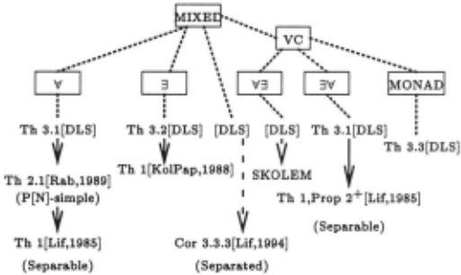
In comparing the different approaches and results con cerning the reduction of circumscriptive theories, we will refer to Figure 1 below, which provides a pictorial view of the subsumption relation between the various theorems and types of theories reduced. DLS refers to our algo rithm, MIXED refers to theories with mixed quantifiers, VC refers to theories which allow variable constants, and MONAD refers to theories with only monadic sentences. In addition, V' and 3 refer to purely universal and ex istential theories, respectively, while V'3 refers to those theories where Skolemization is necessary, and 3V' refers to mixed theories not requiring Skolemization. The solid arrows denote subsumption. In addition there are two broken solid arrows. The arrow pointing towards "Cor 3.3.3" is broken to signify that although the DLS algo rithm in its general form does not fully subsume Corol lary 3.3.3, when specialized appropriately, it does. We discuss this in a later section. The arrow pointing to wards SKOLEM is broken to signify that the DLS algo rithm works for those theories involving Skolemization when the unskolemization step is successful and the al gorithm returns a first-order formula as output. Since, it may not be possible to unskolemize certain theories successfully, there is no complete subsumption of this class.
4 Rabinov requires n-simplicity here.
Positive Results
In addition to the results described in the previous sec tion, observe that the method we propose is also stronger in regard to the following features:
- DLS provides us with a more general approach to existential quantification due to the possibility of allowing Skolemization. Thus it works for combi nations of existential and universal quantifiers. On the other hand, Kolaitis and Papadimitriou consider pure existential formulas, while Lifschitz and Rabi nov consider pure universal theories.
- DLS does not distinguish between theories with variable constants and those without. On the other hand both Rabinov, Kolaitis and Papadimitriou, (and Lifschitz to some extent), restrict their theo ries to those without variable constants. In some cases, Lifschitz's results can reduce theories with variable constants if the theories are separable and no Skolemization is involved. (See the next section for problems DLS has with separated theories).
- DLS permits as input circumscriptive theories with arbitrary numbers of minimized and varied predi cates. This is not the case for Rabinov's result nor for Lifschitz's result pertaining to separated formu las.
- DLS describes how to constructively transform for mulas into the required form.
Negative Results
Note that in the end of Section 2.2 we characterized the class of formulas for which the algorithm fails. Let us now discuss an additional source of weaknesses of the algorithm and a possible way of overcoming those weak nesses.
Observe that the elimination algorithm we deal with is independent of any particular theory. On the other hand, it is well known that second-order quantifiers can sometimes be eliminated when additional information is given.
One good illustrative example originates from the area of modal logics. Namely, McKinsey's axiom is not equiv alent to any first-order formula. Accordingly, our al gorithm fails (see [Szalas, 1993]). However, when one assumes that the accessibility relation is transitive, the elimination is possible, since McKinsey together with transitivity is first-order definable (see [Benthem, 1984]).
The same situation may occur when one computes cir cumscription. Consider the following theorem from [Lif schitz, 1994] (labeled "Cor 3.3.3" in Fig. 1):
Theorem 3.4 If T(P) is a first-order sentence sepa rated w.r.t. P then
Circso(T(P); P; ()) is equivalent to a first-order sen tence. ·
It permits one to deal with any sequences of first order quantifiers provided that the formula is separated. The proof given by Lifschitz is based on a clever move which applies knowledge about the first-order theory one works with. Observe that in Theorem 3.4 the sentence T(P) is assumed to be separated, i.e. it is of the form T1(P)AT2(P), where T1(P) is positive w.r.t. P and T2(P) is negative w.r.t. P. Thus Circso(T1AT2; P; ()) is equivalent to
Since T2(P) is negative w.r.t. P, T2(P) together with q; <Pimply T2(Cl)). Thus when T2(P) is taken into con sideration, one substantially simplifies the second order circumscription into the following second-order formula
The last formula is reducible to a first-order sentence (and is, in fact, in the scope of our algorithm).
The above examples show that the general algorithm we presented can (and should be) tuned to the particular situation it is applied to. Since circumscription is always defined over some first-order theory, moves similar to the method used by Lifschitz above, should be incorporated into the algorithm. If this is done for the case of sep arated theories by slightly modifying the preprocessing phase, then the specialized version of our algorithm sub sumes all previous results concerning the reduction of circumscriptive theories.
4 Complexity of Reduction
Observe that the elimination algorithm we consider, ter minates and is easily mechanizable. Let us now estimate its complexity.
First observe that during phase (3) of the algorithm, the form of the formula to be transformed is 5
and then its form is
after application of the Ackermann lemma.
Thus, if the length of (8) is n, then the length of (9) is less than n 2 · Observe, however, that this worst case occurs when q; has O(n) occurrences in (8). In practical examples, however, the length of (9) is usually O(n) (and often less than the length of ( 8)).
The worst case analysis of steps (1) and (2) shows that the size of the transformed formula can increase exponentially (due to possible transformations between disjunctive and conjunctive normal forms). This, how ever, is again a rare phenomenon- see examples below, in particular Section 5.2 concerning a Kolaitis and Pa padimitriou example.
5 Applying the Algorithm to some Examples
The best way to understand how the algorithm works is to apply it to examples. Due to space limitations, we only apply the algorithm to two examples. A full catalogue of worked examples may be found in [Doherty et al., 1994]. We take a number of liberties in applying the algorithm so as not to drown in details. For example, step (2) in the previous section states that both forms of Ackermann's Lemma should be considered. In the examples, we choose one form and apply the algorithm. This saves considerable space. Also, the simplification phase is omitted unless it can be applied.
5.1 The Birthday Example
Example 5.1 (Birthday Example)
This example contains both existentially quantified and universal formulas. In addition, it contains both unary and binary predicates. Let r(Ab, G) be the theory
where B, F and G are abbreviations for Birthday, Friend and GivesGift, respectively. Here Ab(x, y) has the following intuitive interpretation: "x behaves abnor mally w.r.t. y in the situation when y has a birthday and x is a friend of y". The circumscription of r(Ab, G) with Ab minimized and G varied is
where
5 The second form considered in lemma 2.1 is symmetric to the first one.
In the following, we will reduce
in (11). Negating (15), we obtain
We remove '11 first.
Preprocessing. Replacing r(«P, '11), «P ~ Ab and Ab ~ ~ by their equivalents given by (12)-(14), eliminating ), renaming individual variables and moving existential quantifiers over individual variables to the left, we obtain
Preparation for the Ackermann lemma. (17) is in the form suitable for application of the Ackermann lemma. To see this, we rewrite it as
Application of the Ackermann lemma. Applying the Ackermann lemma to (18), we obtain
We now remove «P in {19).
Preprocessing. (19) is in the form which is the goal of this phase.
Preparation for the Ackermann lemma. Using Proposition 1.1 (8), we replace (19) by
Application of the Ackermann lemma. Applying the Ackermann lemma to (20), we obtain
Simplification. We replace {21) by
Negating (22), we obtain
- is logically equivalent to
which is equivalent to
The first-order formula (25) is logically equivalent to the second-order formula (15). Consequently,
A more informative sentence, equivalent to (25), is
(27), together with the theory r(Ab, G), states that there is exactly one pair of individuals, x and y, such that y has a birthday, x is a friend of y and x does not give a gift toy.
5.2 An Existential Example
[Kolaitis and Papadimitriou, 1988] state
We notice that computing a first-order sen tence equivalent to the circumscription of P in an existential first-order formula tj;(P) seems to increase the size of t/J(P) exponentially, a phe nomenon not observed in the other known cases of first-order circumscription studied in (Lif85]. It would be interesting to determine whether this is inherent to existential first-order formu las, or a particular creation of our proof.
Example 5.2 (Existential Example) In light of the quote above, we take the example used by Kolaitis and Papadimitriou and compare the resulting first-order for mula with that generated by our algorithm. Kolaitis and Papadimitriou apply their reduction technique to the theory
and circumscribe P without varying predicates. The first-order equivalent they obtain is
We apply our reduction algorithm to the same theory and compare the results.
Let r(P) be the theory
The circumscription of r(P) with P minimized without variable predicates is
where
In the following, we will reduce
in (31). Negating (35), we obtain
Preprocessing. Replacing r(~), ~ ~ P and P ~~by their equivalents given by (32)-(34), eliminating :) and renaming individual variables, we obtain
We next move 3xax23z to the left, obtaining
Preparation for the Ackermann lemma. Applying Proposition 1.1 (8) and some standard equivalences, we replace (38) by
Application of the Ackermann lemma. The Acker mann lemma can now be applied to (39) resulting in
Simplification. Applying Proposition 1.1(11) to (39) results in
Negating (41), we obtain
The first-order formula (42) is logically equivalent to the second-order formula (35). Consequently,
Comparing ( 43) with (29), it is easily observed that not only is there a difference in the size of the formulas, but the output appears to make more sense relative to the minimization policy.
6 Conclusion
In this paper, we have presented a general algorithm which transforms second-order formulas into logically equivalent first-order formulas for a large class of second order formulas. The algorithm has been shown to have a number of attractive properties, including a poten tially wide area for practical application. To support this claim, we have provided a detailed description of the algorithms application to the reduction of circum scription axioms. In addition, we have shown that the algorithm, in its general form, provably subsumes nearly all existing results concerning the reduction of circum scription axioms. In contrast to previous results, the algorithm is more constructive in the sense that it pro vides a step-by-step method for transforming a formula and is guaranteed to terminate.
@inproceedings{ijcai1995p194,
  title     = {Computing Circumscription Revisited: Preliminary Report},
  author    = {Doherty, Patrick and Lukaszewicz, Witold and Szalas, Andrzej},
  booktitle = {Proceedings of the Fourteenth International Joint Conference on
               Artificial Intelligence, {IJCAI-95}},
  publisher = {International Joint Conferences on Artificial Intelligence},
  editor    = {Chris S. Mellish},
  pages     = {1502--1507},
  year      = {1995},
  note      = {Non-monotonic Reasoning},
  url       = {https://ijcai.org/proceedings/1995/194},
}
TY - CPAPER TI - Computing Circumscription Revisited: Preliminary Report AU - Doherty, Patrick AU - Lukaszewicz, Witold AU - Szalas, Andrzej T2 - Proceedings of the Fourteenth International Joint Conference on Artificial Intelligence, IJCAI-95 PB - International Joint Conferences on Artificial Intelligence PY - 1995 SP - 1502 EP - 1507 UR - https://ijcai.org/proceedings/1995/194 ER -Copied
Machine-readable versions of this paper, for tools and AI agents:





