
Multiresolution Instance-Based Learning
Proceedings of the Fourteenth International Joint Conference on Artificial Intelligence. Learning. Pages 1233-1241.
© 1995 International Joint Conferences on Artificial Intelligence
Abstract
Instance-based learning methods explicitly remember all the data that they receive. They usually have no training phase, and only at prediction time do they perform computation. Then, they take a query, search the database for similar datapoints and build an on-line local model (such as a local average or local regression) with which to predict an output value. In this paper we review the advantages of instance based methods for autonomous systems, but we also note the ensuing cost: hopelessly slow computation as the database grows large. We present and evaluate a new way of structuring a database and a new algorithm for accessing it that maintains the advantages of instance-based learning. Earlier attempts to combat the cost of instancebased learning have sacrificed the explicit retention of all data, or been applicable only to instancebased predictions based on a small number of near neighbors or have had to re-introduce an explicit training phase in the form of an interpolative data structure. Our approach builds a multiresolution data structure to summarize the database of experiences at all resolutions of interest simultaneously. This permits us to query the database with the same flexibility as a conventional linear search, but at greatly reduced computational cost.
- [Kibler and Aha, 1988] D. Kibler and D. W. Aha, Comparing Instance Averaging and Instance Filtering Learning Algorithms, Proceedings of 3rd European Working Session on Learning, Pitman, 1988
- [Atkeson, 1989] C. G. Atkeson, Using Local Models to Control Move- ment, Proceedings of' Neural Information Processing Systems Con(er- ence, 1989
- [Franke, 1982] R. Franke, Scattered Data Interpolation: Tests of Some Methods, Mathematics fJ(Computation, Vol38, No 157, January 1982.
- [Grosse, 1989] E. Grosse, LOESS: Multivariate Smoothing by Moving Least Squares, Approximation Theory VI, Edited by C. K. Chul, L. L. Schumaker and J. D. Ward , Academic Press, 1989 [Maron and Moore, 1994]
- Maron and A. W. Moore, Hoeffding Races: Accelerating Model Selection Search, Advances in Neural In(ormation Processing Systems 6, 1994
- [Moore, 1990] A. W. Moore, Acquisition of Dynamic Control Knowl- edge for a Robotic Manipulator, Proceedings of' the 7th International Con(erence on Machine Learning, Morgan Kaufmann, 1990
- [Moore et al., 1992] A. W. Moore and D. J. Hill and M.P. Johnson, An Empirical Investigation of Brute Force to choose Features, Smoothers and Function Approximators, Computational Learning Theory and Natu- ral Learning Systems, Volume 3, Edited by S. Hanson and S. Judd and T. Petsche, MIT Press, 1992
- [Omohundro, 1991] S. M. Omohundro, Bumptrees for Efficient Function, Constraint, and Classification Learning, Advances in Neural Information Processing Systems 3, 1991 [
- [Preparata et at., 1985] F. P. Preparata and M. Shamos, Computational Geometry, Springer-Verlag, 1985
- [Quinlan, 1993] J. R. Quinlan, Combining Instance-Based and Model- Based Learning, Machine Learning: Proceedings of the Tenth Interna- tional Conference, 1993
- [Skalak, 1994] D. B. Skalak, Prototype and Feature Selection by Sam- pling and Random Mutation Hill Climbing Algorithms, Machine Learn- ing: Proceedings of the Eleventh International Conference, 1994 [
- [Stanfill et al., 1986] C. Stanfill and D. Waltz, Towards Memory-Based Reasoning, Communications f~( the A CM, 29( 12), 1986
References were extracted automatically from the PDF and may contain errors.
Full text extracted automatically from the PDF; figures, tables and equations may differ. The PDF is the version of record.
1. Introduction
Instance-based learning methods [Stanfill et at., 1986; Atkeson, 1989; Aha et at., 1991; Moore, 1990] are highly flexible, general purpose techniques for making predic tions from earlier data. Instance-based methods (also known as "memory-based" methods or "lazy-learning" methods, and closely related to "case-based" methods) explicitly remember all the data they are shown. Only at prediction time do they perform non-trivial amounts of computation. This behavior differs from more conven tional machine learning algorithms, in which training occurs between the reception of data and prediction. Examples of instance-based methods are nearest neighbor, kernel regression, and locally weighted linear regression. Example of non-instance-based techniques (they have a training phase) are neural networks and decision trees. Instance based methods can sometimes be a preferable form of function approximator. There are three main rea sons for this:
Flexible Inductive Bias
With very little data, a method such as nearest neighbor gives sensible, conservative predictions: it does not wildly extrapolate. But as the amount of data increases, so does the complexity of the function that nearest neighbor can approximate. This contrasts with, for example, multi-layer neural networks that do not by default have this property of representative power increasing locally according to the amount of local data. In the limit, very local methods can learn any piecewise continuous function to arbitrary preci sion (although with high dimensional, uniformly distrib uted input the amount of data to do this can be enormous). For practical use in function approximation, much better instance-based methods than nearest neighbor are avail able that form local linear models, and compute weighted averages of data to remove the noise from predictions (e.g, see [Atkeson, 1989; Grosse, 1989]).
Learning parameters need not be fixed in advance
There are many learning parameters in instance-based algorithms. One of the most important concerns the extent to which the smoothing of noise is traded against goodness of fit. Others include (i) the parameters of a distance metric for determining the similarity between an input point and the query and (ii) the discrete decision of which attributes are relevant. Instance-based methods do not need to decide on these learning parameters in advance. They can use whichever parameters they desire for one prediction and then have the option of using an entirely different set for another prediction. This is of immense use in an autono mous system that is both making new predictions online and tuning its learning parameters online as new data is arriving [Moore et al., 1992]. In contrast, a non-instance based method must choose a parameter set and then train with it. If a different parameter set is later needed then it is necessary for a non-instance-based method to retrain itself (and it is therefore also necessary for it to remember all previous data).
Instance-based can cover the global-local spectrum
Instance-based methods do not necessarily have to be local predictors, based on a small handful of local datapoints. This is particularly important for large num bers of attributes, highly noisy data, and for small data bases. Many of our own applications involve very noisy systems in which the underlying function is non-linear but generally smooth. In these cases the best instance-based function approximator might, for example, use the closest 30% of all datapoints to the query to form its prediction. In some extreme cases, for example if the underlying func tion were nearly linear and local linear regression was in use, this figure might increase to 80% of the datapoints-- essentially a global, not local, function approximator.
The properties described above make instance-based methods particularly desirable for autonomous systems that spend their lives in environments that are not known in advance and in which the designers will not be able to manually tweak the learning parameters during operation.
Unfortunately, instance-based methods have a serious problem. As the database grows large it becomes increas ingly expensive to make predictions. Each prediction involves searching the database to find similar earlier datapoints. This can mean hopelessly slow performance after merely tens of thousands of predictions. Various researchers have attempted to deal with this problem [Aha et al., 1991; Grosse, 1989; Moore, 1990; Skalak, 1994], but, as we will see in Section 7, none in a manner that avoids sacrificing at least one of the benefits of instance based methods described above. This paper describes a new solution, based on a multiresolution hierarchical structuring of data, which retains all the above properties of instance-based learning while providing fast instance based performance. Asymptotically it reduces the cost of a query from linear to logarithmic in the number of datapoints.
2. Kernel Regression
The approach taken in this paper can be applied to a wide variety of instance-based algorithms, but here we will con centrate on one of the most well known examples: Kernel Regression (see, for example, [Franke, 1982]). Assume that datapoints consist of {input, output} pairs such as (xJ,Y 1), (xz,y 2 ), ... (xN,YN) where the inputs are d-element real-valued vectors and the outputs are scalars, and to date we have observed N datapoints. The prediction problem is: given an input vector Xq, which is called the query, how to predict the output yest(xq)?
The k-nearest neighbor solution to this problem would be to find the k datapoints that have input vectors closest to the query and to take the average of the corresponding out put values as ye 81 (xq). Kernel regression uses a similar idea except that a weighted average of all the points in the data base is used, and the points closest to the query are assigned the largest weight. Thus:
where w i is the weight assigned to the ith datapoint in our memory, and is large for points close to the query and almost zero for points far from the query. It is calculated as a decreasing function of Euclidean distance, for example by a gaussian:
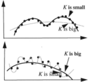
The bigger the parameter K is, the flatter the weight func tion curve is, which means that many memory points con tribute quite evenly to the regression. As K tends to infinity the predictions approach the global average of all points in the database. If the K is very small, only closely neighbor ing datapoints make a significant contribution.
K is an important smoothing parameter for kernel regres sion. If the data is relatively noisy, we expect to obtain smaller prediction errors with a relatively large K. If the data is noise free then a small K will avoid smearing away fine details in the function. This is illustrated in Figure 1.
The drawback of kernel regression is the expense of enu merating all the distances and weights from the memory points to the query. Several methods have been proposed to address this problem, reviewed in Section 7.
3. Multiresolution structuring of datapoints
The main idea of multiresolution instance-based regres sion is grouping. The following figure shows a 2-d input space case. Given a query, based on the distance from each point to the query, we could calculate a weight for every point in the input space.
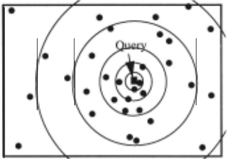
If we split space into several rings as illustrated, we will see that for each group or ring, all the individual weights inside are approximately equal. Assume we have a group with n datapoints in which we know that all weights in the group are close to the same value w. Let the ith member of the group have weight wi = w + f.i where all £is are small. When performing kernel regression we need to accumulate two sums over all datapoints in the database:
The former of these sums will then be divided by the latter. Let us consider how we can compute the contribution to these sums from all the points in our current group. Restricting our attention to summations over the n points in the current group we have
Providing we known, wand Lyi for the current group we can therefore compute an approximation to LwiYi and Lwi in constant time without needing to sum individual mem bers of the group. This approximation to the partial sums is good to the extent that Lf;Yi is small with respect to wLyi and L£i is small with respect to nw.
Kd-trees for grouping
We now understand that if we are given a query, and if someone has structured the set of datapoints into groups for which, relative to the current query, all weights in each group are very similar, then we can compute approxima tions to the sums L, wiyi and L, wi in time proportional to
the number of groups instead of the number of individual datapoints. But how can such a set of groupings be obtained? And how can we ensure that all weights within each grouping are very similar?
We can use a kd-tree [Preparata et al., 1985], enhanced with extra cached information, as an implementation of this grouping idea. A kd-tree is a binary tree that recur sively splits the whole input space into partitions, in a manner similar to a decision tree acting on real-valued inputs. Each node in the kd-tree represents a certain parti tion of the input space; the children of this node denote subsets of the partition. Hence, the root of the kd-tree is the whole input space, while the leaves are the smallest possi ble partitions this kd-tree offers. The tree is built in a man ner that adapts to the local density of input points and so the sizes of partitions at the same level are not necessarily equal to each other.
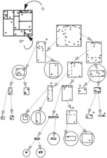
Instead of dividing the input space into rings, we use hyper-rectangles within the kd-tree to implement the grouping idea. The groups are internal nodes of the kdtree. Which nodes are selected for a given query? They are chosen to be nodes that represent hyper-rectangles in input space over which the weight function (relative to the cur rent query) varies little. Hence, at parts of state space with a highly varying weight function (often the part near the query) we use leaves or lower-level internal nodes---small sized partitions. And at parts of state space with little vari ation in the weight function (often the parts far from the query) we use the higher-level internal nodes. This is iiius trated in figure 3.
When the query, Q, is at the top-right corner of the input space in our diagram, the circled nodes in the tree are the groups used for the prediction. The radii of the circles depend on the distances from the hyper-rectangles to the query. For a different query, Q*, we use different group ings, shown by nodes with a * mark.
Kernel Regression Trees Defined
Each node of the kd-tree denotes a hyper-rectangle of input space, and also is defined to contain all datapoints that have input vectors inside this hyper-rectangle. The root node covers the whole of input space and contains all the datapoints. The leaf nodes explicitly record the datapoints that reside in the leaf.
Each node records the hyper-rectangle covered by it. This is defined as the smallest bounding box that contains all the datapoints owned by this node of the tree.
Each non-leaf node has two children representing two dis joint subregions of the parent node. The break between the children is defined by two values. split_d is the split ting dimension, and determines which component of input space (which "attribute") the children will be split upon. split_v determines the numerical value at which each split occurs, The datapoints owned by the left child of a node are those datapoints owned by the node which are less than value split_v in input component split_d. The right child contains the other datapoints.
Finally, each node contains two other pieces of informa tion: n_below, the number of datapoints below the cur rent node, and sum, the sum LYi of all output values of datapoints contained in this node. These are two of the three values needed to compute the contribution of a group to the partial sums in kernel regression. The third compo nent, w, depends upon the location of the query and is determined dynamically in a manner described shortly.
Constructing the kernel regression tree
To construct a tree from a batch of training instances we use a top-down recursive procedure. This is the most stan dard way of constructing kd-trees, described, for example, in [Preparata et at., 1985; Omohundro, 1991]. In this work we use the common variation of splitting a hypercube in the center of the widest dimension instead of at the median point. This method of splitting does not guarantee a bal anced tree, but leads to generally more cubic hyper-rectan gles, which has empirically proved better than other schemes (pathological imbalances are conceivable, but trivial modifications to the algorithm prevent that). The cost of making a tree from N datapoints is O(N log N).
The base case of the recursion occurs when a node is cre ated with Nmin or fewer datapoints. Then those datapoints are explicitly stored in the leaf node. In our experiments Nmin =2.
To incrementally add a new datapoint to the tree, the leaf node containing the point is determined (O(log N) cost). The datapoint is inserted there (and a new subtree is recur sively built if the number of nodes exceeds Nmin). Then all ancestors of the updated node are updated to maintain con sistency in their hyper-rectangles, sum and n_below val ues.
4. Computing the kernel regression sums
Given a query point Xq we are required to compute Lwi and LWiYi, summed over all datapoints in the tree and then divide the latter by the former. This is performed by a top down search over the tree. At each node we make a deci sion between:
- (Cutoff) Treat all the points in this node as one group (a cheap operation) or
- (Recurse) search the children.
We will use the cutoff option if we are confident that all weights inside the node are similar. Given the current query Xq and the hyper-rectangle of the current node it is an easy matter to compute Dmin and Dmax: the minimum and maximum possible distances of any datapoint in this node to the query (computational cost is linear in the num ber of dimensions). From these values one can then com-
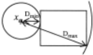
pute the minimum and maximum possible weights wmin and wmax of any datapoints owned by this node, since the weight of a point is a decreasing function of distance to the query. We thus decide if wmin and Wmax are close enough to warrant the cut-off option.
The search is thus a recursive procedure which returns two values: sum-weights and sum-wy. If the cutoff option is taken, then estimate the weight of all datapoints as ~ = (wmin+wmax)/2 and return:
If the cutoff option is not taken, recursively compute sum weights and sum-wy for the left and right children, and then return:
sum-weights= sum-weights( left)+ sum-weights( right) sum-wy = sum-wy(left) + sum-wy(right)
5. Search Cutoffs
Section 3 described how we can make our approximation arbitrarily accurate by bounding the maximum deviation we will permit from the true weight estimate with a value Emax > 0 and then making Emax arbitrarily small. Thus the simplest cutoff rule in the kd-tree search would be to cutoff if Wmax- Wmin < Emax· It is easy to show that this guaran tees that the total sum of absolute deviations ILE) is less than NJ€max I 2 where NT is the number of points in the tree. There are, however, other possible cutoff criteria which provide arbitrary accuracy in the limit, but which, when used as an approximation, have more satisfactory properties.
The simple cutoff rule does not take into account that a larger total error will occur if the node contains very many points than if the node contains only a few points. It does also not account for the fact that in a practical case we are less concerned about the absolute value of the sum of devi ations IL£il but rather the size of IL£il relative to the sum of the weights LWi. Some simple analysis reveals a cutoff criterion to satisfy both of these intuitions. Cutoff only if
where N 8 is the number of datapoints below the current node. Simple algebra reveals that this guarantees
where G is the number of groups finally used in the search (and thus G < Ny, hopefully considerably less). Notice that this cutoff rule requires us to know :Ew i in advance, which of course we do not. Fortunately the sum of weights obtained so far in the search can be used as a valid lower bound, and so the real algorithm makes a cutoff if:
where 't is a system constant.
6. Experiments and results
Let us review the performance of the multiresolution method in comparison to kernel regression. In the first experiment we use a trigonometric function of two inputs with added noise: xi = uniformly generated random vector with all components between 0 and 100 and Yi = a function of xi (which ranges between 0 and 100 in height), with gaussian noise of standard deviation 10.
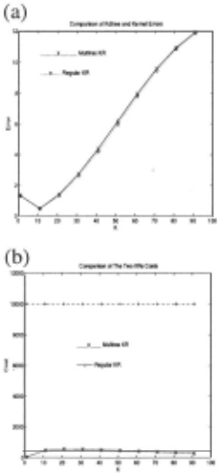
10,000 datapoints were generated. Experiments were run for different values of kernel width K. In all experiments, the cutoff threshold 'twas 0.005. Figure 4a shows the test set error on 1000 test points for both regular kernel regres sion ("Regular KR") and multiresolution kernel regression ("Multires KR") graphed for different values of K. The values are very close, indicating that multires KR is pro viding, for a wide range of kernel widths, a very close approximation to regular KR. Figure 4b shows the compu tational cost (in terms of the summations that dominate the cost of KR) of the two methods. Regular KR sums all points, and so is a constant 10,000 in cost. Multires KR is substantially cheaper for all values of K, but particularly so for very small and very large values.
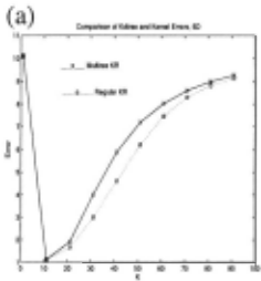
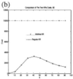
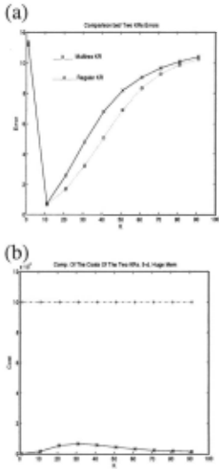
Figures 5a and 5b show corresponding figures for a similar trigonometric function of five inputs. This still shows sim ilar prediction performance as regular KR. The cost is still always less than regular KR, but in the worst case the com putational saving is only a factor of three (when K = 40, multires KR cost = 3,200). This is not an especially impressive result. However, for any fixed dimensionality and kernel width, costs rise sub-linearly (in principle loga rithmically) with the number of datapoints. To check this, we ran the same set of experiments for a dataset of ten times the size: 100,000 points. The results, in Figure 6, show that with this large increase in data, the effectiveness
'
'
'
Figure 6: The same experiment as Figure 5, except with ten times the amount of data: I 00,000 datapoints
of multires KR becomes more apparent. For example, con sider the K = 40 case. With 100,000 datapoints instead of 10,000, the cost is only increased from 3,200 to 5,700 while the cost of regular KR (of course) increased from 10,000 to 100,000.
Investigating the t threshold parameter
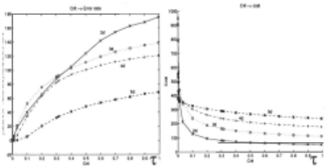
Next, we will examine the effect of the 't parameter on the behavior of the algorithm. As 't is increased we expect the computational cost to be reduced, but at the expense of the accuracy of the predictions in comparison to the regular KR. The results in Figure 7 agree with this expectation: the left hand graph shows that for 2-d, 3-d, 4-d and 5-d datasets (each with 10,000 points) the proportional error between multires and regular regression increases with 't. The right hand graph shows a corresponding decrease in computational cost.
""
Figure 7. (Upper) the relative accuracy and (lower) the computational cost of multi res KR against 't--the cutoff threshold.
Real datasets
In another experiment, we ran multires KR on data from several real-world and robot-learning datasets. Further details of the datasets can be found in [Maron and Moore, 1994]. They include an industrial packaging process for which the slowness of prediction had been a reasonable cause for concern. Encouragingly, multires KR speeds up prediction by a factor of 100 with no discernible difference in prediction quality between multires and regular KR. This and other results are tabulated below. The costs and RMS values given are averages taken over an independent test set. Notably, the datasets with the least savings were pool, which had few datapoints, and robot, which was high dimensional.
| Domain | Number Points | Dimen- sion | KR Cost | MRes Cost | KR rms err | MRes rms err |
|---|---|---|---|---|---|---|
| I Energy | 12144 | 15-d | 12144 | 1232.9 | 11.687 | 1.690 |
| Package | 32000 | 3-d | 32000 | 289.0 | 6.07 | 6.09 |
| Pool | 213 | 3-d | 213 | 50.7 | 2.125 | 2.123 |
| Protein | 4664 | 3-d | 4664 | 383.8 | 1.036 | 1.106 |
| Robot | 871 | 14-d | 871 | 225 | 6.354 | 6.976 |
High dimensional, non-uniform data
Our final experiment concerned the question of how well the method performs if the number of input variables is rel atively large, but if the attributes are not independent. For example, a common scenario in robot learning is for the input vectors to be embedded on a lower-dimensional manifold. We performed two experiments, each with 9 inputs and 10,000 datapoints. In the first experiment, the components of the input vectors were distributed uni formly randomly. In the second experiment the input vec tors were distributed on a non-linear 2-d manifold of the 9d input space. The results were:
| 9-d uniform | 9-d inputs on 2d manifold | |
|---|---|---|
| I Regular KR cost | 110,000 | 10,uuu |
| Multires KR cost | 3,100 | 430 |
| Regular KR mean testset error | 13.07 | 1.06 |
| Multires KR mean testset error | 13.08 | 1.15 |
The results indicate that, as would be expected, the cost advantage of multires KR is not large (a factor of 3) for 9-d uniform inputs, but is far better if the inputs are distributed within a lower-dimensional space.
7. Related Work and Discussion
There has not been room in this paper to discuss a number of additional ftexibilities that multires KR provides. Once the kd-tree structure is built, it is possible to make different queries with not only different kernel widths K , but also different Euclidean distance metrics, with subsets of attributes ignored, or with some other distance metrics such as Manhattan. It is also possible to apply the same technique with different weight functions and for classifi cation instead of regression.
It should be remembered that although we have succeeded in reducing the cost of instance-based learning, there are other methods (outlined below) in the literature for doing so. Why might Multires be preferable? This depends upon the extent to which the application needs the following advantages of instance based learning described in Section 1:
- Flexibility to work throughout the local/global spec trum.
- The ability to make predictions with different parameters without needing a retraining phase.
Multires provides for both. No other software method, to our knowledge, does. There is, however, the simple hard ware alternative of using a fast enough computer. The stan dard kernel regression method can be parallelized with full efficiency.
Kd-trees have frequently been used in instance-based learning methods for nearest neighbor searching or for range searching [Preparata et al., 1985]. The range-search solution to kernel regression is to find all points in the kd tree that have a significant weight, and then only sum together the weighted components of those points. This is only practical if the kernel width K is small. If it is large, all the datapoints may have a significant weight, but only a small local variation in weight. Range searching would sum all the points individually. Multires would visit only relatively large intermediate nodes (because the weight variation is locally low) and so would still be cheap. Even in cases of small kernel widths and large amounts of data the multiresolution method can be preferable to the range search method because it may not need to search all the way down to the leaf nodes.
Another solution to the cost of instance-based learning is editing (or prototypes): most datapoints are forgotten and only particularly representative ones are used (e.g. [Kibler and Aha, 1988; Skalak, 1994]). Kibler and Aha extended this idea further by allowing datapoints to represent local averages of sets of previously-observed datapoints. This can be effective, and unlike range-searching can be appli cable even for wide kernel widths. However, the degree of local averaging must be decided in advance: unlike Mul tires, queries cannot occur with different kernel widths without rebuilding the prototypes. A second occasional problem is that if we require very local predictions, the prototypes must either lose local detail by averaging, or else all the datapoints are stored as prototypes.
There are interesting parallels between prototypes and Multires. The intermediate nodes of the kd-tree can be thought of as fabricated prototypes, summarizing all the data below them.
Decision trees and kd-trees have been previously used to cache local mappings in the tree leaves [Grosse, 1989; Moore, 1990; Omohundro, 1991; Quinlan, 1993] . These algorithms provide fast access once the tree is built, but a new structure needs to be built each time new learning parameters are required. Furthermore, unlike the multires olution method, the resulting predictions from the tree have substantial discontinuities between boundaries. Only in [Grosse, 1989] is continuity enforced, but at the cost of tree-size, tree-building-cost and prediction-cost all being exponential in the number of input variables.
Dimensionality is a weakness of Multires. Diminishing returns set in above approximately 10 dimensions if the data is distributed uniformly. This is an inherent problem for which no solution seems likely because uniform data in high dimensions will have almost all datapoints almost exactly the same distance apart, and a useful notion of locality breaks down.
This paper discussed an efficient implementation of kernel regression. We are applying exactly the same algorithm to locally weighted polynomial regression, in which a predic tion fits a local polynomial to minimize the locally weighted sum squared error. The only difference is that each node of the kd-tree stores the regression design matrices of all points below it in the tree. This permits fast pre diction and also fast computation of confidence intervals and analysis of variance information.
Multires as described here is only applicable to numeric features. An interesting avenue for future work would be ways to extend the method to binary or symbolic features.
8. Conclusion
Instance based methods make use of a database of multidi mensional data. Multiresolution instance-based methods provide a means for performing queries quickly, even when the amount of data is enormous. An important mes sage of this paper is that for efficient accessing of large instance bases (or case bases, or memory-bases) it is not necessary to resort to throwing data away. Intelligent structuring is an alternative.
Acknowledgement
We wish to thank the IJCAI reviewers for insightful and useful comments. This work was support by a research gift from 3M corporation and an NSF Reserach Initiation Award.
@inproceedings{ijcai1995p159,
  title     = {Multiresolution Instance-Based Learning},
  author    = {Deng, Kan and Moore, Andrew W.},
  booktitle = {Proceedings of the Fourteenth International Joint Conference on
               Artificial Intelligence, {IJCAI-95}},
  publisher = {International Joint Conferences on Artificial Intelligence},
  editor    = {Chris S. Mellish},
  pages     = {1233--1241},
  year      = {1995},
  note      = {Learning},
  url       = {https://ijcai.org/proceedings/1995/159},
}
TY - CPAPER TI - Multiresolution Instance-Based Learning AU - Deng, Kan AU - Moore, Andrew W. T2 - Proceedings of the Fourteenth International Joint Conference on Artificial Intelligence, IJCAI-95 PB - International Joint Conferences on Artificial Intelligence PY - 1995 SP - 1233 EP - 1241 UR - https://ijcai.org/proceedings/1995/159 ER -Copied
Machine-readable versions of this paper, for tools and AI agents:





