
Practical PAC Learning
Proceedings of the Fourteenth International Joint Conference on Artificial Intelligence. Learning. Pages 1169-1176.
© 1995 International Joint Conferences on Artificial Intelligence
Abstract
We present new strategies for "probably approximately correct" (pac) learning that use fewer training examples than previous approaches. The idea is to observe training examples one-at-a-time and decide "on-line" when to return a hypothesis, rather than collect a large fixed-size training sample. This yields sequential learning procedures that pac-learn by observing a small random number of examples. We provide theoretical bounds on the expected training sample size of our procedure - but establish its efficiency primarily by a series of experiments which show sequential learning actually uses many times fewer training examples in practice. These results demonstrate that paclearning can be far more efficiently achieved in practice than previously thought.
- [Aha, et al., 1991] D. Aha, et al. Instance-based learning al- gorithms. Machine Learning, 6(1):37-66, 1991.
- [Bartlett and Williamson, 1991] P . Bartlett and R. William- son. Investigating the distributional assumptions of the pac learning model. In COLT-91, pages 24-32, 1991.
- [Baum and Haussler, 1989] E. Baum and D. Haussler. What size net gives valid generalization? Neural Computation, 1:151-160, 1989.
- [Benedek and Itai, 1988] G. Benedek and A. Itai. Learnabil- ity by fixed distributions. In COLT-88, pages 80-90, 1988.
- [Blumer, et al., 1989] A. Blumer, et al. Learnability and the Vapnik-Chervonen. dimension. JACM, 36:929-965, 1989.
- [Breiman, et al., 1984] L. Breiman, et al. Classification and Regression Trees. Wadsworth, Belmont, CA, 1984.
- [Clancey, 1985] W. Clancey. Heuristic classification. Artifi- cial Intelligence, 27:289-350, 1985.
- [Dennis and Schnabel, 1983] J. Dennis and R. Schnabel. Nu- merical Methods for Unconstrained and Nonlinear Equa- tions. Prentice-Hall, Englewood Cliffs, N J, 1983.
- [Duda and Hart, 1973] R. Duda and P. Hart. Pattern Clas- sification and Scene Analysis. Wiley, New York, 1973.
- [Ehrenfeucht, et al., 1989] A. Ehrenfeucht, et al. A general lower bound on the number of examples needed for learn- ing. Information and Computation, 82:247-261, 1989.
- [Haussler, 1990] D. Haussler. Probably approximately cor- rect learning. In AAAI-90, pages 1101-1108, 1990.
- [Haussler, 1992] D. Haussler. Decision theoretic generaliza- tions of the PAC model. Inf. and Comp., 100:78-150, 1992.
- [le Cun, et al., 1989] Y. le Cun, et al. Backpropagation ap- plied to handwritten zip code recognition. Neural Compu- tation, 1:541-551, 1989.
- [Linial, et al., 1991] N. Linial, et al. Results on learnability and the Vapnik-Chervonenkis dimension. Information and Computation, 90:33-49, 1991.
- [Littlestone, 1989] N. Littlestone. From online to batch learning. In COLT-89, pages 269-284, 1989.
- [Oblow, 1992] E. Oblow. Implementing Valiant's learnability theory using random sets. Mach. Learn., 8:45-73, 1992.
- [Schaffer, 1994] C. Schaffer. A conservation law for general- ization performance. In Proceedings ML-94, 1994.
- [Schuurmans and Greiner, 1995] D. Schuurmans and R. Greiner. Sequential PAC learning. In COLT-95, 1995.
- [Schuurmans, 1995] D. Schuurmans. Effective Classification Learning. PhD thesis, U. Toronto, Computer Sci., 1995.
- [Shawe-Taylor, et al., 1993] J. Shawe-Taylor, et al. Bound- ing sample size with the Vapnik-Chervonenkis dimension. Discrete Applied Mathematics, 42:65-73, 1993.
- [Valiant, 1984] L. Valiant. A theory of the learnable. CACM, 27(11):1134-1142, 1984.
- [Vapnik and Chervonenkis, 1971] V. Vapnik and A. Chervo- nenkis. On the uniform convergence of relative frequencies of events to their probabilities. Theory of Probability and its Applications, 16(2):264-280, 1971.
- [Wald, 1947] A. Wald. Sequential Analysis. Wiley, 1947.
- [Weiss and Kulikowski, 1991] S. Weiss and C. Kulikowski. Computer Systems that Learn. Morgan Kaufmann, 1991.
References were extracted automatically from the PDF and may contain errors.
Full text extracted automatically from the PDF; figures, tables and equations may differ. The PDF is the version of record.
1 Introduction
We consider the standard problem of learning an accu rate classifier from examples: given a target classifica tion scheme c : X -t Y defined on a domain X, we are interested in observing a sequence of training examples ((x1 , c(x1)), ... , (xt, c(xt))) and producing a hypothesis h: X-+ Y that agrees with con as much of the domain as possible. Here we adopt the standard batch training pro tocol, where after a finite number of training examples the learner must produce a hypothesis h, which is then tested ad infinitum on subsequent training examples.
In practice, domain objects can be represented in many different ways (e.g., boolean or real-valued vectors, or structured descriptions like strings, graphs, terms, etc.), and so too can hypotheses (e.g., decision trees, neural networks, nearest neighbor classifiers, etc.). How ever, regardless of the specific representation used, the central question is always how best to extrapolate the classifications of a few domain objects to an accurate classification scheme over the entire domain.
Motivation: Classification learning is by far the most studied in machine learning research. The immense in terest in this problem arises from the fact that classi fication itself is an important subtask in many appli cations - in fact, comprising the central function of
Russell Greiner
Siemens Corporate Research Princeton, N J 08540, USA greiner~scr.siemens.com
most expert systems [Clancey, 1985]. The importance of learning in this context is that we often lack the requisite knowledge needed to specify an appropriate classifier, and yet have access to many correctly clas sified examples. In such situations, we can attempt to exploit the wealth of available data to overcome inadequate prior knowledge - and hence, use learn ing as an effective classifier synthesis tool. In fact, there are numerous examples where learning systems have produced classifiers that outperform the best avail able "hand-coded" systems, e.g., [le Cun, et al. , 1989; Weiss and Kulikowski, 1991].
Although empirical research tends to examine the per formance properties of particular hypothesis guessing strategies on specific domains, the underlying goal of classification learning research is to uncover whatever general principles might underly the effective extrapola tion of training object classifications to entire domains. However, it has often been observed that there really is no such thing as a "general purpose" extrapolation strat egy [Schaffer, 1994] - a particular strategy performs well on a specific application only by fortuitous predisposi tion: it just happens to "guess right" on unseen domain objects, whether by prior knowledge or luck. To guaran tee success, one must supply prior constraints.
The current trend towards theoretical analysis in ma chine learning represents a fundamental shift in emphasis away from discovering "universal" extrapolation strate gies, towards explicitly acknowledging the role played by prior constraints in yielding successful extrapolation. The role of a theoretical analysis is not to prescribe prior knowledge/constraints, but to determine the best that can be achieved given whatever is known beforehand.
1.1 Pac-learning theory
The most influential analysis of classification learning is the theory of "probably approximately correct" (pac) learning introduced by Valiant [1984]. Rather than spec ulate about the mechanisms that might underly "gen eral purpose" classification learning, Valiant's idea was to characterize those situations where successful learning could be provably achieved, and where it is demonstrably impossible.
Problem: Pac-learning theory adopts an "i.i.d. ran dom examples" model of the learning situation, which assumes domain objects are independently generated by a fixed distribution Px and labelled according to a fixed target concept c : X --+ { 0, 1}. Under this model, the er ror of a hypothesis h: X--+ {0, 1} with respect to c and Px is given by Px{h(x) # c(x)}. Here we consider the difficulty of meeting the so-called pac-criterion: produc ing a hypothesis h with error at most f, with probability at least 1 -IS, for specified accuracy and reliability pa rameters f and IS. Of course, the difficulty of achieving this criterion depends on how much we know about c and Px beforehand. Pac-learning theory adopts a model of prior knowledge where we assume the target concept c belongs to some known class C, but nothing is known about the domain distribution Px. Given this model, we naturally consider what can be achieved in the "worst case, distribution-free" sense:
Definition 1 (Pac-learning problem) A learner L solves the pac-learning problem (X, C, t, IS) {or "pac(t, IS) learns C ") if, for any c in C and P x, L produces a hy pothesis h such that P x { h ( x) # c( x)} :S t with probability at least 1- IS (over possible training sequences).
For example, we might be interested in solving the problem (X = JR 10 , C = halfspace, f = 0.01, IS= 0.05), where domain objects are described by 10 real-valued attributes, the target concept is known to be some linear halfspace of JR 10 , and we wish to produce a hypothesis with 1% error with probability at least 95%. Our goal is to solve these learning problems as efficiently as possi ble - i.e., using a minimum of data and computational resources. The primary focus of this paper is on improv ing the data-efficiency of pac-learners, rather than their computational-efficiency.
Results: Some of the most important technical results ofpac-learning theory concern the data resources needed to solve pac-learning problems. Intuitively, it should take more training examples to pac-learn a complex con cept class than a simple one, since it is harder to disam biguate possible target concepts from a complex class. The question is: how can one measure the representa tional complexity of a concept class C so as to precisely determine the number of training examples needed to pac(t, IS)-learn C? It turns out that just such a measure is provided by the Vapnik-Chervonenkis (VC) dimension of C: 1 Ehrenfeucht et al. [1989] have shown that, for any concept class C with vc(C) = d, the minimum number of training examples needed by any learner to pac( f, IS) learn Cis at least tEHKv(C, t, IS)= max { ~2 1 , 1 ;' In;}}. Furthermore, there is a simple fixed-sampZe-size learn ing procedure, F, that always meets this lower bound to within constant and log factors, and hence learns with near-optimal data-efficiency; see Figure 1. In particu lar, Blumer et al. [1989] have shown that for any 2 con- Procedure F (C,t,o)
1 The VCdimension measures how "fine grained" Cis by the maximum number of domain objects C can independently label [Vapnik and Chervonenkis, 1971]. This is an abstract combinatorial measure which applies to arbitrary domains and concept classes. Moreover, it often gives intuitive results (e.g., the class of halfspace concepts on IR" is defined by n + 1 "free parameters" and also has a VCdimension of n + 1).
2 C must satisfy certain (benign) measurability constraints [Blumer, et al., 1989], which we will assume throughout.
COLLECT Tp( C, t, o) training examples, sufficient to eliminate all t-had concepts from C with prob. at least 1-8.
RETURN any h E C that correctly classifies every example.
Figure 1: Procedure F
cept class C, TBEHw(C, t, IS) =max { 8 ,d log2 1 , 3 , ~ log2 t} random training examples are sufficient to ensure F pac(t,IS)-learns C, where d = vc(C) . (This result has since been improved by Shawe-Taylor et al. [1993] to TsTAB(C,t,IS)=,( 1 !J€) (2dln%+Int).) Overall, these are powerful results as they characterize the necessary and sufficient training sample sizes needed to pac-learn any concept class C in terms of a "tight" linear function of its VCdimension.
1.2 Issue
However, despite these impressive results, pac-learning theory has arguably had little direct impact on the actual practice of machine learning. Why? Beyond criticisms of certain modelling assumptions (e.g., noise-free examples, bivalent classifications, etc.- which actually have been addressed the pac-framework, cf. [Haussler, 1992]), the most prevalent criticism of pac-learning theory is that the actual numbers of training examples it demands are far too large to be practical.
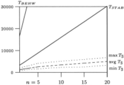
Example: Consider the (X = JR 10 , C = halfspaces , t = 0.01, IS= 0.05) problem mentioned earlier. Noting that vc(C) = 11, we can simply use TBEHw to determine a sufficient sample size for Procedure F. But here we find TBEHw demands 91,030 training examples! (Even the improved TsTAB demands 15,981 examples in this case.) This seems like an outrageous number given the appar ently modest parameter settings. Moreover, these results compare poorly to the empirical "rule of thumb" that, for a concept class defined by w free parameters, roughly T,humb = ~ training examples are needed to achieve an er ror off [Baum and Haussler, 1989]. Applied here, T,humb demands only 1, 100 training examples - an order of magnitude fewer than TsTAB· (Of course, this rule of thumb comes with no guarantees, but it does give an indication of how many training examples practitioners would deem "reasonable" for this problem.) Further more, TBEHw and TsTAB are orders of magnitude larger than the best known lower bound tEHKv, which demands only 32 training examples in this case! See Table 1 in Section 3 for a direct comparison.
This shows that, although the theoretical upper and lower bounds are tight up to constant and log factors, they give results that are orders of magnitude apart in practice. This has drastic consequences for the applica bility of the theory, since in practice it is often training data, not computation time, that is the critical resource. I. e., cutting the training sample size in half would be a significant improvement in most applications, even if this came with a slight increase in overall computation time.
The apparent inefficiency of pac-learning has lead to much speculation about the sources of difficulty. The predominant "folk wisdom" is that the large sample sizes follow from the worst case nature of the pac guarantees [Haussler, 1990] - that is, the worst case bounds are inherently unreasonable because they must take into account "pathological" domain distributions and target concepts which force large training sample sizes (moreover, the argument continues, these patho logical situations do not arise in "typical" applications). In fact, this belief motivates much research that makes distributional assumptions in order to improve data efficiency, e.g., [Benedek and Itai, 1988; Aha, et al., 1991; Bartlett and Williamson, 1991]. However, notice that this line of reasoning is actually quite weak: First of all, no-one can demonstrate that these "pathological" situations really exist (for this would be tantamount to improving the lower bound tEHKv)- Secondly, it is clear from the previous example that the current bounds are loose, and can likely be substantially improved - e.g. , TsTAB and tEHKv differ by roughly a factor of 64ln ~Approach: In this paper we investigate an alternative view: perhaps the simplistic (collect; find) learning pro cedure F is not particularly data-efficient. This raises the obvious question of whether alternative learning strate gies might be more data-efficient than F. Here we investi gate sequential learning procedures that observe training examples one-at-a-time and autonomously decide "on line" when to stop training and return a hypothesis. The idea is that we should be able to detect situations where an accurate hypothesis can be reliably returned, even before the sufficient sample size bounds have been reached (e.g. , we might detect that C has been reduced to a single possible target). The hope is that, in this way, we can significantly reduce the number of training examples observed, while still meeting the exact same pac-criterion as before: namely, that an €-accurate hy pothesis be returned with probability at least 1--J for any target concept c E C and distribution P x. An underlying assumption here is that we are willing to incur a slight computational penalty to obtain a significant improve ment in data-efficiency. This is motivated by the fact that training data is usually the most critical resource in practical learning applications.
The remainder of this paper develops a few simple sequential learning procedures that (i) are correct pac learners, (ii) are provably data-efficient, and (iii) use many times fewer training examples in empirical case studies.
2 Sequential pac-learning
A sequential learner L consists of a stopping rule TL, that maps training sequences to stopping times, and a hypothesizer H L, that maps finite training sequences to hypotheses. Our basic strategy for constructing sequen tial pac-learners is to take an arbitrary consistent hy pothesizer H for C (which produces hypotheses hE C that correctly classify every observed training example), collect H's hypotheses, and test these against subsequent training examples until one proves to have sufficiently small error. The main challenge is finding an appropri ate stopping rule that guarantees the pac-criterion, while observing as few training examples as possible.
Procedure R ( C, f., 8, H)
FIX a sequence { 8;} r' such that L 8; = 8. Call H to obtain an initial hypothesis ho .
SEQUENTIALLY observe training examples (xt, y1), t = 1, 2, ... :
IF current hypothesis h; makes a mistake, call H to obtain a consistent hi+! (drop h;, begin testing h;+!)·
RETURN current hypothesis h; if it correctly classifies ~ ln -h consecutive training examples.
Figure 2: Procedure R
Note that, in general, a sequential learner observes a random, rather than fixed, number of training examples. Thus, to compare the data-efficiency of our approach with previous techniques, we must compare a distribu tion of sample sizes to a fixed number. There are anum ber of ways one could do this, but we focus on what is arguably the most natural measure: comparing the av erage (i.e., expected) training sample size of a sequential learner with the fixed sample size demanded by previous approaches to solve the same pac-learning problem.
Obvious approach: Perhaps the most obvious strat egy for sequential pac-learning is based on the idea of repeated significance testing: test a series of hypothe ses generated by H until one correctly classifies a suffi cient number of consecutive training examples; see Pro cedure R in Figure 2. 3 Although this is a plausible ap proach (which, in fact, works well in practice), it is hard to prove reasonable bounds on R's expected sample size. The problem is that R rejects "good enough" hypotheses with high probability, and yet takes a long time to do so (i.e., R rejects hypotheses of error f with probability 1 - c5, but this takes ~ expected time). Thus, if H pro duces a series of "borderline" hypotheses, R will take a long time to terminate (expected time about~' which is not very good). Fortunately, there is a better approach.
Better approach: Here we introduce a novel learning procedure, S (Figure 3), which is also based on repeated significance testing, but avoids the apparent inefficiency of R's "survival testing" approach. S is based on two ideas: First, instead of throwing away H 's hypotheses after a single mistake, S saves hypotheses and contin ues testing them until one proves to have small error. Second, S identifies accurate hypotheses by using a se quential probability ratio test (sprt) [Wald, 1947] to test each candidate "on-line" (in parallel); Figure 4. Thus, S never rejects a potentially acceptable hypothesis, and quickly identifies any sufficiently accurate candidate.
Procedure S is a correct pac-learner in the exact same sense as F: The key property of S is that its call to sprt eventually accepts any ~-good hypothesis with proba bility 1 (wp1), but only accepts an f-bad hypothesis h; with probability at most c5; . This implies that S even tually halts wpl, and returns an f-good hypothesis with Procedure S ( C, t, 8, H)
3 Variants of Procedure R have been proposed by many au thors in the past [Linial, et al., 1991; Oblow, 1992], primarily to achieve "nonuniform" pac-learning. However, the goals of nonuniform pac-learning fundamentally differ from what we are trying to accomplish here (see Footnote 6).
FIX a sequence { 8; = ~ H" and a constant "' > 1. Initialize a list of hypotheses with ho, obtained by calling H .
SEQUENTIALLY observe training examples (xt, Yt), t = 1, 2, ... :
IF the most recent hypothesis h; makes a mistake, call H to add a new, consistent hypothesis hi+! to the list .
TEST all hypotheses in the list (in parallel) by calling sprt(h;(x):;6c(x), -!z, t, 8;, 0)
for each h; (when generated).
RETURN the first generated hypothesis hj sprt accepts.
Figure 3: Procedure S
probability at least 1 - J, for any target concept c E C and domain distribution Px (thus, achieving the exact same worst case pac-guarantees as F). 4 This property also allows us to prove a reasonable upper bound on the average number of training examples S observes for any target concept c E C and domain distribution Px .
Theorem 1 For f > 0, J > 0, and any (well behaved) concept class C with vc(C) = d: using a consistent hy pothesizer H for C and any constant"' > 1, ProcedureS observes an average training sample size of at most
for any target concept c E C and distribution Px.
Although this is a crude bound, it is interesting to note that it scales the same as TsEHw and TsTAB · Moreover, this bound actually beats TsEHw and TsTAB for small val ues of J [Schuurmans, 1995] . However, as shown below, S actually performs much better in practice than any bounds we can prove about its performance. Since this is not a possibility for fixed-sample-sized approaches, we expectS to perform much better than TsEHw and TsTAB in practical applications.
Before demonstrating S's advantage in empirical tests, we first note that there are inherent limits to the data efficiency even of sequential learning.
Theorem 2 For sufficiently small f and J, and any con cept class C with vc(C) = d 2 2: any learner that al ways observes (for any fixed c E C and Px) an average training sample size less than
cannot meet the pac( f, J) -criterion for all c E C and P x.
Notice that this lower bound scales the same as tEHxv in terms off and vc(C) -which shows that no new con cept classes become pac-learnable merely by considering a sequential over fixed-sample-size approach.
4 Provided vc( C) < oo (details omitted). Proofs of all results mentioned in this paper (and more) are outlined in [Schuurmans and Greiner, 1995]. Complete details appear in [Schuurmans, 1995].
Procedure sprt (4>(x), a, r, 8acc, 8rej)
FoR boolean random variable q)(x), test
Haec: Px{4>(x)=1}:::; a vs. Hrej : Px{4>(x)=1} 2: r, with: -probability of deciding Haec given Hrej bounded by 8acc, - probability of deciding H rej given H ace bounded by 8 reJ . SEQUENTIALLY observe q)1 = q)(xt), t = 1, 2, ... ;monitoring: St = 2:::=1 4>iln ~ + (1- 4>i)ln ~=~ · RETURN "accept" if ever St 2: In 1/8acc·
RETURN "reject" if ever St :::; In 8rej.
Figure 4: Procedure sprt
3 Empirical efficiency
Although the theoretical advantage we can demonstrate for Sis only slight, we expectS to perform much better in practice than any bounds we can prove about its perfor mance. This is because S's actual data-efficiency in any particular case study is determined by the specific case at hand, and not by the worst case situation (or, worse yet, what we can prove about the worst case situation) . In fact, in empirical studies, S proves to be far more efficient than any bounds. we can prove about its per formance, and many times more efficient than TsEHw or TsTAB · This is easily demonstrated by a simple example.
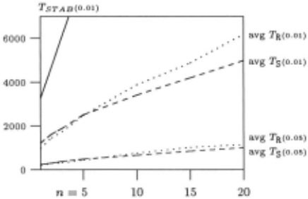
Illustration: We tested Procedure S on the problem (X=1Rn,C=halfspaces,f=0.01,J=0.05) with the fol lowing setup: Training objects were generated accord ing to a uniform distribution on [-1, 1)n and labelled by a fixed target halfspace (defined by a "diagonal" hyper plane passing through the origin on with norm directed towards 1 n). The constant "' was set to 3.14619 (so that ,._ 1 ~ 1 n,. =K), and we supplied S with a hypothesizer H that finds consistent halfspace concepts. 5 We ran Pro cedure S 100 times for n = 10 and obtained the results shown in Table 1. Notice that S's average training sam ple size of 3, 402 is about 5 times smaller than T sTAs , 27 times smaller than TsEHw, and only about 3 times larger than T.humb· It is important to emphasize that S obtains these empirical sample size improvements while maintaining the exact same worst case pac-guarantees as before (that an f-accurate hypothesis is returned with probability at least 1 - J). These results are in fact rep resentative over the entire range of parameter settings: S's empirical advantage actually improves for increased problem dimension n (Figure 5), and is maintained at higher accuracy and reliability levels [Schuurmans, 1995]. Overall, S appears to be pac-learning with near-practical data-efficiency in this example.
Interestingly, S also outperforms the simplistic proce dure R on this problem. Figure 6 shows that, R performs nearly as well as S on easy problems (low dimension, ac curacy, reliability), butS's advantage grows significantly as these parameters are scaled up.
5 Specifically, we used the BFGS secant optimization pro cedure [Dennis and Schnabel, 1983] with a "relaxation" ob jective function [Duda and Hart, 1973] .
Explanations: These results demonstrate a clear ad vantage for sequential over fixed-sample-size learning: we solve the exact same pac-learning problem using far fewer training examples in this case. Of course these pre ceding results are anecdotal, and it is tempting to explain away the advantage as a mere artifact of the specific ex perimental setup. However, we have found that these experimental results are, in fact, quite robust.
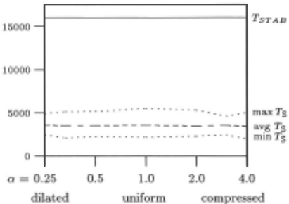
First, the previous experiment only tested a single do main distribution (uniform), which could happen to be a particularly "easy" one for S. To counter this claim, we repeated the experiment with various domain distribu tions to see if any could seriously affect S's performance. In particular, we considered three different transforma tions of the uniform( -1, 1]n distribution: spherical (non linear compression towards origin), pyramidal (compres sion from opposite corners towards hyperplane), and ac cretive (translation towards discrete points in { -1, l}n). Surprisingly, none of these transformations had any no ticeable effect on S's performance [Schuurmans, 1995]; as demonstrated in Figure 7 for the pyramidal case.
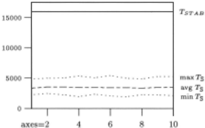
A second reason for S's advantage might be that the specific target concept (diagonal halfspace) is a partic ularly "easy" one for S - i.e., H could somehow be biased to guess similar hypotheses. However, this is eas ily shown not to be the case: We repeated the original experiment on 10 different target halfspaces, each suc cessively closer to "axis-parallel," and found that none of these made any appreciable difference; Figure 8.
Third, it could be the case that the class of halfspaces concepts happens to be "easy" among classes with com parable VCdimension. This turns out to be partly true: We have been able to construct alternative con cept classes which force S to observe slightly more train ing examples; see Figure 9. However, we have yet to de vise any concept class (with the same VCdimension) that can even double S's original performance on halfspaces. In fact , S 's performance often improves for different con cept classes (particularly finite ones). Overall, it appears that halfspaces is not a remarkably hard or easy class for a given VCdimension. ·
Another explanation of S's advantage over F is that TsrAB might possibly be a gross overestimate of the true worst case situation (which seems likely, given the gap between T sTAB and tEHKv). Of course, this means that any current advantage enjoyed by S could potentially be overcome by future improvements to TsrAB - but notice that we can enjoy S's improved performance im mediately, without having to wait for theoreticians to improve the bounds. (Ensuring the correctness of F re quires one to prove some bound is sufficient; this is not a requirement for Procedure S since its correctness is completely decoupled from its efficiency.)
A final explanation of S's advantage is that sequential learning might be inherently more efficient than fixed sample-size learning. Clearly, since the sequential ap proach generalizes the fixed-sample-size approach, it can be no worse than F. The question is how substantial an advantage can be obtained in principle? This is left largely unanswered by our empirical results, and remains an interesting open topic for future research.
| For (X = JR 10 , C = halfspaces, f.= 0.01, 8 = 0.05): | |||
| Sufficient: | TBEHW | 91,030 | |
| Improved: | TsTAB | 15,981 | |
| Folklore: | Tthumb | ~ | 1, 100 |
| Necessary: | tEHKV | 32 | |
| After 100 trials, Procedure S used: | |||
| avg Ts | 3,402 | ||
| maxTg | 5,155 | ||
| minTs | 2,267 | ||
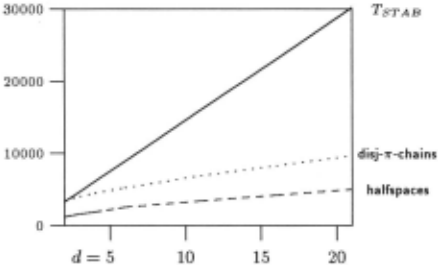
Advantages: Despite the empirical nature of these re sults, sequential learning holds many clear advantages over fixed-sample-size learning for solving pac-learning problems: First, the sequential approach decouples the actual data-efficiency of a pac-learner from the precise bounds we can prove about its performance a priori. Thus, the actual data-efficiency of a sequential learner depends on the specific case at hand, not on what we can prove about the worst case situation. Consequently, the sequential approach automatically takes adva.ntage of beneficial situations like "easy" target concepts and domain distributions [Oblow, 1992), or a "good" hypoth esizer that makes lucky guesses -- without the system designer having to explicitly notice that these beneficial situations exist a priori! More importantly, the true worst case data-efficiency of sequential learning depends on the true worst case convergence properties of the con cept class, not on the particular bounds we happen to be able to prove at the time (i.e., if bad concepts are eliminated sooner than proven bounds, then S automat ically stops sooner). So, in effect, we are able to exploit the optimal worst case bounds right now, even though we are unable to prove exactly what they are.
Computation: We also note that Procedure S only in troduces reasonable compu.tational overhead over Pro cedure F; and in fact, is often more computationally efficient than R! Although, at first glance, S appears to be extremely space-inefficient, this rarely amounts to a significant expense in practical applications. The point is that, in practice, it is the task of finding consistent hypotheses (calling H) that takes most of the work - storing hypotheses once found (updating statistics, etc.) does not require much overhead in comparison. Conse quently, R is often slower than S (even though it uses less space) simply because R tends to call H more often.
4 Additional results
Special cases: We have obtained even stronger results in slightly restricted settings [Schuurmans and Greiner, 1995]. For example, a variant of Procedure S can serve as a sequential "mistake bounded to pac" conversion procedure that is provably more efficient than Little stone's fixed-sample-size procedure [Littlestone, 1989] (and which uses 30 times fewer training examples in em pirical tests). We also obtain stronger improvements for the case of distribution specific pac-learning (where we assume the learner knows Px, but not the target concept c E C). Notice that a sequential approach is still possi ble in this case; and, in fact, a variant of Procedure S can pac-learn concept spaces ( C, P x) using 5 times fewer training examples than the best known fixed-sample-size procedure developed in [Benedek and Itai, 1988].
Range of applicability: Beyond improving data efficiency, sequential learning is also applicable to a much wider range of pac-learning problems than fixed-sample size learning. For example, Procedure S can be directly applied to "nearest neighbor" and "decision-tree" hy pothesizers (like CART [Breiman, et al., 1984]) which implicitly consider concept classes of infinite VCdimen sion. No fixed-sample-size bound can ever be sufficient in these cases, and yet Procedure S can be applied to pac-learn these classes "as is." The only catch is that we can no longer place a uniform upper bound on S's expected training sample size. 6
5 Conclusion
Research directions: There are numerous directions for future research. First, since our empirical results address "artificial" learning problems, it would be in teresting to test these procedures on "real world" data sets (e.g., as contained in the UCI repository of machine learning databases) to verify that the same empirical ad vantages can be realized there. Another important re search direction is to extend our techniques to deal with classification noise, which remains the main barrier be tween the results presented here and real applications. Finally, one can also consider a slightly different learning scenario which perhaps has more practical applications than pac-learning: rather than first fixing the accuracy and reliability parameters and then determining a suffi cient sample size, it is much more natural to take a fixed sample size, fix a reliability parameter, and produce an estimate of the accuracy achieved by the learner's final hypothesis. In this regard, we are currently investigat ing a variant of Procedure S which produces hypotheses with small (but reliable!) error estimates.
Contributions: We have described a novel pac-learning procedure, S, that uses far fewer training examples than previous approaches. Procedure S is, in effect, generic test procedure that can pac-learn arbitrary con cept classes C (with finite VCdimension), provided only that we can supply a hypothesizer H that produces con sistent concepts from C. This procedure introduces little computational overhead, and yet substantially reduces the number of training examples needed to pac-learn in practice - as demonstrated in numerous case studies where S used many times fewer training examples than the previous best known approaches, while still main taining the exact same worst case pac-guarantees.
In a way, these results exploit the empirical advan tage demonstrated by practical learning algorithms over the theoretical bounds, to improve the efficiency of pac learning. Overall, our results show how pac-learning can be far more efficiently achieved in practice than previ ously thought - countering the claim that pac-learning can never be feasibly achieved in real applications.
Acknowledgments
Thanks to Steven Shapiro for his help with the imple mentations.
6 It is important not to confuse the idea of sequential with nonuniform pac-learning [Linial, et al., 1991; Oblow, 1992]. Although nonuniform pac-learning procedures also use "on-line" stopping rules very similar to R, they do not share the same theoretical advantages shown for S. Sequen tial pac-learning seeks to obtain a uniform improvement in data-efficiency for all cases permitted by our prior knowledge, whereas nonuniform pac-learning sacrifices data-efficiency in some situations to obtain an improvement in others. These two concerns are in fact orthogonal.
@inproceedings{ijcai1995p151,
  title     = {Practical PAC Learning},
  author    = {Schuurmans, Dale and Greiner, Russell},
  booktitle = {Proceedings of the Fourteenth International Joint Conference on
               Artificial Intelligence, {IJCAI-95}},
  publisher = {International Joint Conferences on Artificial Intelligence},
  editor    = {Chris S. Mellish},
  pages     = {1169--1176},
  year      = {1995},
  note      = {Learning},
  url       = {https://ijcai.org/proceedings/1995/151},
}
TY - CPAPER TI - Practical PAC Learning AU - Schuurmans, Dale AU - Greiner, Russell T2 - Proceedings of the Fourteenth International Joint Conference on Artificial Intelligence, IJCAI-95 PB - International Joint Conferences on Artificial Intelligence PY - 1995 SP - 1169 EP - 1176 UR - https://ijcai.org/proceedings/1995/151 ER -Copied
Machine-readable versions of this paper, for tools and AI agents:





