
A Study of Cross-Validation and Bootstrap for Accuracy Estimation and Model Selection
Proceedings of the Fourteenth International Joint Conference on Artificial Intelligence. Learning. Pages 1137-1144.
© 1995 International Joint Conferences on Artificial Intelligence
Abstract
We review accuracy estimation methods and compare the two most common methods: crossvalidation and bootstrap. Recent experimenta l results on artificial data and theoretical results in restricted settings have shown that for selecting a good classifier from a set of classifi ers (model selection), ten-fold cross-validation may be better than the more expensive leaveone-out cross-validation. We report on a largescale experiment-ove r half a million runs of C4.5 and a Naive-Bayes alg orithm-to estimate the effects of different parameters on these a lgorithms on real-world datasets . For crossvalidation, we vary the number of folds and whether the folds are stratified or not; for bootstrap, we vary the number of bootstrap samples. Our results indicate that for real-word datasets simil ar to ours, the best method to use for model selection is ten-fold stratified cross validation, even if computation power allows using more folds.
- Bailey, T . L. & Elkan, C. (1993), Estimating the ac- curacy of learned concepts, in "Proceedings of In- ternational Joint Conference on Artificial Intelli- gence", Morgan Kaufmann Publishers, pp. 895-900. IJCAI
- Breiman, L. & Spector , P. (1992), "Submodel selection and evaluation in regression. the x-random case", International Statistical Review 60(3), 291-319.
- Breiman, L., Friedman, J . H., Olshen, R. A. & Stone, C. J. (1984), Classification and Regression Trees , Wadsworth International Group.
- Efron , B. (1983), "Estimating the error rate of a pre- diction rule: improvement on cross-validation", Journal of the American Statistical Association 78(382), .316-330.
- Efron, B. & Tibshirani, R. (1993), An introduction to the bootstrap, Chapman & Hall.
- Jain , A. K., Dubes, R. C. & Chen, C. (1987), "Boot- strap techniques for error estimation", IEEE trans- actions on pattern analysis and machine intelli- gence PAMI-9(5) , 628-633.
- Kohavi, R., John, G., Long, R., Manley, D. & Pfleger, K. (1994), MLC++: A machine learn- ing library in C++, in "Tools with Artifi- cial Intelligence", IEEE Computer Society Press, pp. 740-743 . Available by anonymous ftp from: starry.Stanford.EDU:pub/ronnyk/rnlc/ toolsrnlc. ps . Link
- Langley, P., Iba, W . & Thompson, K . (1992), An anal- ysis of bayesian classifiers, in "Proceedings of the tenth national conference on artificial intelligence" , AAAI Press and MIT Press, pp. 223-228.
- Murphy, P. M. & Aha, D. W. (1994), UCI repository of machine learning databases, For information con- tact ml-repository@ics .uci.edu .
- Quinlan, J. R. {1993), C4.5: Programs for Machine Learning, Morgan Kaufmann, Los Altos, California.
- Schaffer, C. (1994), A conservation law for generalization performance, in "Machine Learning: Proceedings of the Eleventh International Conference", Morgan Kaufmann, pp. 259-265.
- Shao, J. ( 1993), "Linear model seletion via cross- validation", Journal of the American Statistical As- sociation 88( 422), 486-494.
- Weiss, S.M. (1991), "Small sample error rate estimation for k-nearest neighbor classifiers", IEEE Transac- tions on Pattern Analysis and Machine Intelligence 13(3), 285-289.
- Weiss , S. M. & Indurkhya, N. (1994), Decision tree pruning : Biased or optimal, in "Proceedings of the twelfth national conference on artificial intel- ligence", AAAI Press and MIT Press, pp. 626-632.
- Wolpert , D. H. (1992), "Stacked generalization", Neural Networks 5 , 241-259.
- Wolpert, D. H. (1994a), Off-training set error and a pri- ori distinctions between learning algorithms, Tech- nical Report SFI TR 94-12-123, The Sante Fe In- stitute.
- Wolpert, D. H. (1994b), The relationship between PAC, the statistical physics framework, the Bayesian framework, and the VC framework, Technical re- port, The Santa Fe Institute, Santa Fe, NM .
- Zhang, P. (1992), "On the distributional properties of model selection criteria", Journal of the American Statistical Association 87( 419), 732-737 .
References were extracted automatically from the PDF and may contain errors.
Full text extracted automatically from the PDF; figures, tables and equations may differ. The PDF is the version of record.
1 Introduction
It can not be emphasized enough that no claim whatsoever is being made in this paper that all algorithms are equivalent in practice, in the real world. In particular, no claim is being made that one should not use cross-validation in the real world. - Wolpert {1994a}
Estimating the accuracy of a classifier induced by su pervised learning algorithms is important not only to predict its future prediction accuracy, but also for choos ing a classifier from a given set (model selection), or combining classifiers (Wolpert 1992) . For estimating the final accuracy of a classifier, we would like an estimation method with low bias and low variance. To choose a classifier or to combine classifiers, the absolute accura cies are less important and we are willing to trade off bias for low variance, assuming the bias affects all classifiers similarly (e. g., estimates are 5% pessimistic) .
A longer version of the paper can be retrieved by anony mous ftp to starry.stanford.edu:pub/ronnyk/accEst-long.ps
In this paper we explain some of the assumptions made by the different estimation methods, and present con crete examples where each method fails. While it is known that no accuracy estimation can be correct all the time (Wolpert 1994b, Schaffer 1994), we are inter ested in identifying a method that is well suited for the biases and trends in typical real world datasets.
Recent results, both theoretical and experimental, have shown that it is not always the case that increas ing the computational cost is beneficial, especially if the relative accuracies are more important than the exact values. For example, leave-one-out is almost unbiased, but it has high variance, leading to unreliable estimates (Efron 1983) . For linear models, using leave-one-out cross-validation for model selection is asymptotically in consistent in the sense that the probability of selecting the model with the best predictive power does not con verge to one as the total number of observations ap proaches infinity (Zhang 1992, Shao 1993).
This paper is organized as follows. Section 2 describes the common accuracy estimation methods and ways of computing confidence bounds that hold under some as sumptions. Section 3 discusses related work comparing cross-validation variants and bootstrap variants. Sec tion 4 discusses methodology underlying our experiment. The results of the experiments are given Section 5 with a discussion of important observations. We conclude with a summary in Section 6.
2 Methods for Accuracy Estimation
A classifier is a function that maps an unlabelled in stance to a label using internal data structures. An in ducer, or an induction algorithm, builds a classifier from a given dataset . CART and C4.5 (Breiman, Friedman, Olshen & Stone 1984, Quinlan 1993) are decision tree in ducers that build decision tree classifiers. In this paper , we are not interested in the specific method for inducing classifiers, but assume access to a dataset and an inducer of interest.
Let V be the space of unlabelled instances and Y the set of possible labels . Let X = V x Y be the space of labelled instances and D = { x1, x2, ... , Xn} be a dataset (possibly a multiset) consisting of n labelled instances, where x; = (v; E V, y; E Y). A classifier C maps an unla belled instance v E V to a label y E Y and an inducer I maps a given dataset D into a classifier C. The notation I(D, v) will denote the label assigned to an unlabelled in stance v by the classifier built by inducer I on dataset D, i.e., I(D, v) = (I(D))(v). We assume that there exists a distribution on the set of labelled instances and that our dataset consists of i.i.d. (independently and identically distributed) instances. We consider equal misclassifica tion costs using a 0/1 loss function, but the accuracy estimation methods can easily be extended to other loss functions .
The accuracy of a classifier C is the probability of correctly classifying a randomly selected instance, i.e., ace = Pr(C(v) = y) for a randomly selected instance (v, y) E X, where the probability distribution over the instance space is the same as the distribution that was used to select instances for the inducer's training set. Given a finite dataset, we would like to estimate the fu ture performance of a classifier induced by the given in ducer and dataset. A single accuracy estimate is usually meaningless without a confidence interval; thus we will consider how to approximate such an interval when pos sible. In order to identify weaknesses, we also attempt to identify cases where the estimates fail.
2.1 Holdout
The holdout method, sometimes called test sample esti mation, partitions the data into two mutually exclusive subsets called a training set and a test set, or holdout set. It is common to designate 2/3 of the data as the training set and the remaining 1/3 as the test set. The training set is given to the inducer, and the induced classifier is tested on the test set. Formally, let Dh, the holdout set, be a subset of D of size h, and let Dt be D \ Dh. The holdout estimated accuracy is defined as
where rS(i,j) = 1 if i = j and 0 otherwise. Assuming that the inducer's accuracy increases as more instances are seen, the holdout method is a pessimistic estimator because only a portion of the data is given to the inducer for training. The more instances we leave for the test set, the higher the bias of our estimate; however, fewer test set instances means that the confidence interval for the accuracy will be wider as shown below.
Each test instance can be viewed as a Bernoulli trial: correct or incorrect prediction. Let S be the number of correct classifications on the test set, then S is dis tributed binomially (sum of Bernoulli trials). For rea sonably large holdout sets, the distribution of S/h is ap proximately normal with mean ace (the true accuracy of the classifier) and a variance of ace* (1- acc)/h. Thus , by De Moivre-Laplace limit theorem, we have
where z is the (1+!)/2-th quantile pointofthe standard normal distribution. To get a 1001 percent confidence interval, one determines z and inverts the inequalities. Inversion of the inequalities leads to a quadratic equation in ace, the roots of which are the low and high confidence points:
The above equation is not conditioned on the dataset D; if more information is available about the probability of the given dataset, it must be taken into account.
The holdout estimate is a random number that de pends on the division into a training set and a test set. In random subsampling, the holdout method is re peated k times, and the estimated accuracy is derived by averaging the runs. The standard deviation can be estimated as the standard deviation of the accuracy es timations from each holdout run.
The main assumption that is violated in random sub sampling is the independence of instances in the test set from those in the training set. If the training and test set are formed by a split of an original dataset, then an over-represented class in one subset will be a under represented in the other. To demonstrate the issue, we simulated a 2/3, 1/3 split of Fisher's famous iris dataset and used a majority inducer that builds a classifier pre dicting the prevalent class in the training set . The iris dataset describes iris plants using four continuous fea tures, and the task is to classify each instance (an iris) as Iris Setosa, Iris Versicolour, or Iris Virginica. For each class label, there are exactly one third of the instances with that label (50 instances of each class from a to tal of 150 instances); thus we expect 33.3% prediction accuracy. However, because the test set will always con tain less than 1/3 of the instances of the class that was prevalent in the training set, the accuracy predicted by the holdout method is 27.68% with a standard deviation of 0.13% (estimated by averaging 500 holdouts).
In practice, the dataset size is always finite, and usu ally smaller than we would like it to be. The holdout method makes inefficient use of the data: a third of dataset is not used for training the inducer.
2.2 Cross-Validation, Leave-one-out, and Stratification
In k-fold cross-validation, sometimes called rotation esti mation, the dataset D is randomly split into k mutually exclusive subsets (the folds) D1, D2, ... , Dk of approx imately equal size. The inducer is trained and tested k times; each time t E {1, 2, ... , k}, it is trained on V \ Vt and tested on Vt. The cross-validation estimate of accuracy is the overall number of correct classifica tions, divided by the number of instances in the dataset . Formally, let V(i) be the test set that includes instance x; = (v;, y;) , then the cross-validation estimate of accu racy
The cross-validation estimate IS a random number that depends on the division into folds . Complete cross-validation is the average of all (m/k) possibil ities for choosing mj k instances out of m, but it is usually too expensive. Except for leave-one-one (n-fold cross-validation), which is always complete, k-fold cross validation is estimating complete k-fold cross-validation using a single split of the data into the folds. Repeat ing cross-validation multiple times using different splits into folds provides a better Monte-Carlo estimate to the complete cross-validation at an added cost. In strati fied cross-validation, the folds are stratified so that they contain approximately the same proportions of la bels as the original dataset.
An inducer is stable for a given dataset and a set of perturbations, if it induces classifiers that make the same predictions when it is given the perturbed datasets .
Proposition 1 (Variance in k-fold CV)
Given a dataset and an inducer. If the inducer is stable under the perturbations caused by deleting the instances for the folds in k-fold cross-validation, the cross-validation estimate will be unbiased and the vari ance of the estimated accuracy will be approximately acccv · (1- acccv)/n, where n is the number of instances in the dataset.
Proof If we assume that the k classifiers produced make the same predictions, then the estimated accuracy has a binomial distribution with n trials and probability of success equal to the accuracy of the classifier. I
For large enough n, a confidence interval may be com puted using Equation 3 with h equal to n, the number of instances .
In reality, a complex inducer is unlikely to be stable for large perturbations, unless it has reached its maximal learning capacity. We expect the perturbations induced by leave-one-out to be small and therefore the classifier should be very stable. As we increase the size of the perturbations, stability is less likely to hold: we expect stability to hold more in 20-fold cross-validation than in 10-fold cross-validation and both should be more stable than holdout of 1/3. The proposition does not apply to the resubstitution estimate because it requires the in ducer to be stable when no instances are given in the dataset.
The above proposition helps understand one possible assumption that is made when using cross-validation: if an inducer is unstable for a particular dataset under a set of perturbations introduced by cross-validation, the ac curacy estimate is likely to be unreliable. If the inducer is almost stable on a given dataset, we should expect a reliable estimate. The next corollary takes the idea slightly further and shows a result that we have observed empirically: there is almost no change in the variance of the cross-validation estimate when the number of folds is varied.
Corollary 2 (Variance in cross-validation)
Given a dataset and an inducer. If the inducer is sta ble under the perturbations caused by deleting the test instances for the folds in k-fold cross-validation for var ious values of k, then the variance of the estimates will be the same.
Proof The variance of k-fold cross-validation in Propo sition 1 does not depend on k. I
While some inducers are likely to be inherently more stable, the following example shows that one must also take into account the dataset and the actual perturba tions.
Example 1 (Failure of leave-one-out)
Fisher's iris dataset contains 50 instances of each class, leading one to expect that a majority inducer should have accuracy about 33%. However, the combination of this dataset with a majority inducer is unstable for the small perturbations performed by leave-one-out. When an instance is deleted from the dataset, its label is ami nority in the training set; thus the majority inducer pre dicts one of the other two classes and always errs in clas sifying the test instance. The leave-one-out estimated accuracy for a majority inducer on the iris dataset is therefore 0%. Moreover, all folds have this estimated ac curacy; thus, the standard deviation of the folds is again 0%, giving the unjustified assurance that the estimate is stable. I
The example shows an inherent problem with cross validation that applies to more than just a majority in ducer. In a no-information dataset, where the label val ues are completely random, the best an induction algo rithm can do is predict majority. Leave-one-out on such a dataset with 50% of the labels for each class and a majority inducer (the best possible inducer) would still predict 0% accuracy.
2.3 Bootstrap
The bootstrap family was introduced by Efron and is fully described in Efron & Tibshirani (1993) . Given a dataset of size n, a bootstrap sample is created by sampling n instances uniformly from the data (with re placement). Since the dataset is sampled with replace ment, the probability of any given instance not being chosen after n samples is (1- 1/n)n ~ e- 1 ~ 0.368; the expected number of distinct instances from the original dataset appearing in the test set is thus 0.632n. The f0 accuracy estimate is derived by using the bootstrap sam ple for training and the rest of the instances for testing. Given a number b, the number of bootstrap samples, let f0; be the accuracy estimate for bootstrap sample i. The .632 bootstrap estimate is defined as
where ace, is the resubstitution accuracy estimate on the full dataset (i.e., the accuracy on the training set). The variance of the estimate can be determined by com puting the variance of the estimates for the samples.
The assumptions made by bootstrap are basically the same as that of cross-validation, i.e., stability of the al gorithm on the dataset: the "bootstrap world" should closely approximate the real world. The .632 bootstrap fails to give the expected result when the classifier is a perfect memorizer (e. g. , an unpruned decision tree or a one nearest neighbor classifier) and the dataset is com pletely random, say with two classes. The resubstitution accuracy is 100%, and the f0 accuracy is about 50%. Plugging these into the bootstrap formula, one gets an estimated accuracy of about 68.4%, far from the real ac curacy of 50%. Bootstrap can be shown to fail if we add a memorizer module to any given inducer and adjust its predictions. If the memorizer remembers the training set and makes the predictions when the test instance was a training instances, adjusting its predictions can make the resubstitution accuracy change from 0% to 100% and can thus bias the overall estimated accuracy in any direction we want.
3 Related Work
Some experimental studies comparing different accuracy estimation methods have been previously done, but most of them were on artificial or small datasets. We now describe some of these efforts.
Efron (1983) conducted five sampling experiments and compared leave-one-out cross-validation, several variants of bootstrap, and several other methods. The purpose of the experiments was to "investigate some related es timators, which seem to offer considerably improved es timation in small samples." The results indicate that leave-one-out cross-validation gives nearly unbiased esti mates of the accuracy, but often with unacceptably high variability, particularly for small samples; and that the .632 bootstrap performed best.
Breiman et al. (1984) conducted experiments using cross-validation for decision tree pruning. They chose ten-fold cross-validation for the CART program and claimed it was satisfactory for choosing the correct tree. They claimed that "the difference in the cross-validation estimates of the risks of two rules tends to be much more accurate than the two estimates themselves."
Jain, Dubes & Chen (1987) compared the performance of the f0 bootstrap and leave-one-out cross-validation on nearest neighbor classifiers using artificial data and claimed that the confidence interval of the bootstrap estimator is smaller than that of leave-one-out . Weiss (1991) followed similar lines and compared stratified cross-validation and two bootstrap methods with near est neighbor classifiers. His results were that stratified two-fold cross validation is relatively low variance and superior to leave-one-out.
Breiman & Spector (1992) conducted a feature sub set selection experiments for regression, and compared leave-one-out cross-validation, k-fold cross-validation for various k, stratified k-fold cross-validation, bias corrected bootstrap, and partial cross-validation (not discussed here). Tests were done on artificial datasets with 60 and 160 instances . The behavior observed was: (1) the leave-one-out has low bias and RMS (root mean square) error, whereas two-fold and five-fold cross validation have larger bias and RMS error only at models with many features ; (2) the pessimistic bias of ten-fold cross-validation at small samples was significantly re duced for the samples of size 160; (3) for model selection, ten-fold cross-validation is better than leave-one-out .
Bailey & Elkan (1993) compared leave-one-out cross validation to .632 bootstrap using the FOIL inducer and four synthetic datasets involving Boolean concepts . They observed high variability and little bias in the leave-one-out estimates, and low variability but large bias in the .632 estimates.
Weiss and Indurkyha (Weiss & Indurkhya 1994) con ducted experiments on real-world data to determine the applicability of cross-validation to decision tree pruning. Their results were that for samples at least of size 200, using stratified ten-fold cross-validation to choose the amount of pruning yields unbiased trees (with respect to their optimal size) .
4 Methodology
In order to conduct a large-scale experiment we decided to use C4.5 and a Naive-Bayesian classifier. The C4.5 algorithm (Quinlan 1993) is a descendent of ID3 that builds decision trees top-down. The Naive-Bayesian clas sifier (Langley, lba & Thompson 1992) used was the one implemented in M.CC++ (Kohavi, John, Long, Manley & Pfleger 1994) that uses the observed ratios for nominal features and assumes a Gaussian distribution for contin uous features. The exact details are not crucial for this paper because we are interested in the behavior of the accuracy estimation methods more than the internals of the induction algorithms. The underlying hypothe sis spaces-decision trees for C4.5 and summary statis tics for Naive-Bayes- are different enough that we hope conclusions based on these two induction algorithms will apply to other induction algorithms.
Because the target concept is unknown for real-world concepts, we used the holdout method to estimate the quality of the cross-validation and bootstrap estimates. To choose a set of datasets, we looked at the learning curves for C4.5 and Naive-Bayes for most of the super vised classification datasets at the UC Irvine repository (Murphy & Aha 1994) that contained more than 500 instances (about 25 such datasets) . We felt that a min imum of 500 instances were required for testing. While the true accuracies of a real dataset cannot be computed because we do not know the target concept, we can esti mate the true accuracies using the holdout method. The "true" accuracy estimates in Table 1 were computed by taking a random sample of the given size, computing the accuracy using the rest of the dataset as a test set, and repeating 500 times.
We chose six datasets from a wide variety of domains, such that the learning curve for both algorithms did not flatten out too early, that is, before one hundred instances . We also added a no information dataset , rand, with 20 Boolean features and a Boolean random label. On one dataset, vehicle, the generalization accu racy of the Naive-Bayes algorithm deteriorated by more than 4% as more instances were given. A similar phe nomenon was observed on the shuttle dataset. Such a phenomenon was predicted by Schaffer and Wolpert (Schaffer 1994, Wolpert 1994b), but we were surprised that it was observed on two real-world datasets.
To see how well an accuracy estimation method per forms, we sampled instances from the dataset (uniformly without replacement), and created a training set of the desired size. We then ran the induction algorithm on the training set and tested the classifier on the rest of the instances in the dataset. This was repeated 50 times at points where the learning curve was sloping up. The same folds in cross-validation and the same samples in bootstrap were used for both algorithms compared.
5 Results and Discussion
We now show the experimental results and discuss their significance. We begin with a discussion of the bias in the estimation methods and follow with a discussion of the variance. Due to lack of space, we omit some graphs for the Naive-Bayes algorithm when the behavior is ap proximately the same as that of C4.5.
5.1 The Bias
The bias of a method to estimate a parameter (} is de fined as the expected value minus the estimated value. An unbiased estimation method is a method that has zero bias. Figure 1 shows the bias and variance of k-fold cross-validation on several datasets (the breast cancer dataset is not shown).
The diagrams clearly show that k-fold cross-validation is pessimistically biased, especially for two and five folds . For the learning curves that have a large derivative at the measurement point, the pessimism in k-fold crossvalidation for small k's is apparent. Most of the esti mates are reasonably good at 10 folds and at 20 folds they are almost unbiased.
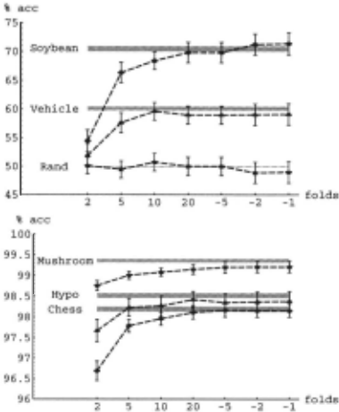
Stratified cross-validation (not shown) had similar be havior, except for lower pessimism. The estimated accu racy for soybean at 2-fold was 7% higher and at five-fold, 4.7% higher; for vehicle at 2-fold, the accuracy was 2.8% higher and at five-fold, 1.9% higher. Thus stratification seems to be a less biased estimation method.
Figure 2 shows the bias and variance for the .632 boot strap accuracy estimation method. Although the .632 bootstrap is almost unbiased for chess, hypothyroid, and mushroom for both inducers, it is highly biased for soy bean with C4.5, vehicle with both inducers , and rand with both inducers. The bias with C4.5 and vehicle is 9.8%.
5.2 The Variance
While a given method may have low bias, its perfor mance (accuracy estimation in our case) may be poor due to high variance. In the experiments above, we have formed confidence intervals by using the standard de viation of the mean accuracy. We now switch to the standard deviation of the population, i.e., the expected standard deviation of a single accuracy estimation run. In practice, if one does a single cross-validation run, the expected accuracy will be the mean reported above, but the standard deviation will be higher by a factor of .;50, the number of runs we averaged in the experiments.
| Dataset | no. of attr. | sample-size / total size | no. of categories | duplicate instances | C4.5 | Naive-Bayes |
|---|---|---|---|---|---|---|
| Breast cancer | 10 | 50/699 | 2 | 8 | 91.37±0.10 | 94.22±0.10 |
| Chess | 36 | 900/3196 | 2 | 0 | 98.19±0.03 | 86.80±0.07 |
| Hypothyroid | 25 | 400/3163 | 2 | 77 | 98.52±0.03 | 97.63±0 .02 |
| Mushroom | 22 | 800/8124 | 2 | 0 | 99.36±0.02 | 94.54±0.03 |
| Soybean large | 35 | 100/683 | 19 | 52 | 70.49±0 .22 | 79.76±0.14 |
| Vehicle | 18 | 100/846 | 4 | 0 | 60.11±0.16 | 46.80±0.16 |
| Rand | 20 | 100/3000 | 2 | 9 | 49.96±0.04 | 49.90±0 .04 |
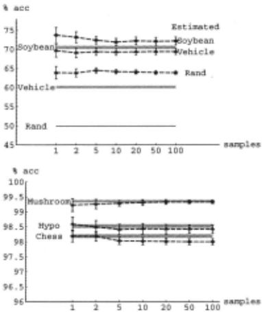
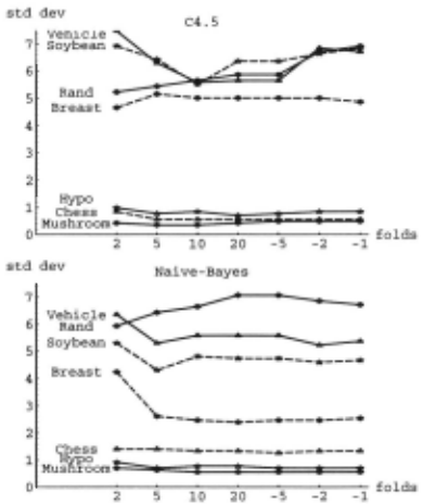
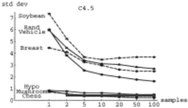
In what follows, all figures for standard deviation will be drawn with the same range for the standard devi ation: 0 to 7.5%. Figure 3 shows the standard devia tions for C4.5 and Naive Bayes using varying number of folds for cross-validation. The results for stratified cross-validation were similar with slightly lower variance. Figure 4 shows the same information for .632 bootstrap.
Cross-validation has high variance at 2-folds on both C4.5 and Naive-Bayes. On C4.5, there is high variance at the high-ends too-at leave-one-out and leave-two out-for three files out of the seven datasets. Stratifica tion reduces the variance slightly, and thus seems to be uniformly better than cross-validation, both for bias and vanance.
6 Summary
We reviewed common accuracy estimation methods in cluding holdout , cross-validation, and bootstrap, and showed examples where each one fails to produce a good estimate. We have compared the latter two approaches on a variety of real-world datasets with differing charac teristics.
Proposition 1 shows that if the induction algorithm is stable for a given dataset, the variance of the cross validation estimates should be approximately the same, independent of the number offolds. Although the induc tion algorithms are not stable, they are approximately stable. k-fold cross-validation with moderate k values (10-20) reduces the variance while increasing the bias. As k decreases (2-5) and the sample sizes get smaller, there is variance due to the instability of the training sets themselves, leading to an increase in variance. This is most apparent for datasets with many categories, such as soybean. In these situations, stratification seems to help, but repeated runs may be a better approach.
Our results indicate that stratification is generally a better scheme, both in terms of bias and variance, when compared to regular cross-validation. Bootstrap has low variance, but extremely large bias on some problems. We recommend using stratified ten-fold cross-validation for model selection.
Acknowledgments We thank David Wolpert for a thorough reading of this paper and many interesting dis cussions. We thank Tom Bylander, Brad Efron, Jerry Friedman, Rob Holte, George John, Pat Langley, Rob Tibshirani, and Sholom Weiss for their helpful com ments and suggestions. Dan Sommerfield implemented the bootstrap method in M.CC++. All experiments were conducted using M.CC++, partly partly funded by ONR grant N00014-94-1-0448 and NSF grants IRI-9116399 and IRI-9411306.
@inproceedings{ijcai1995p147,
  title     = {A Study of Cross-Validation and Bootstrap for Accuracy Estimation and Model Selection},
  author    = {Kohavi, Ron},
  booktitle = {Proceedings of the Fourteenth International Joint Conference on
               Artificial Intelligence, {IJCAI-95}},
  publisher = {International Joint Conferences on Artificial Intelligence},
  editor    = {Chris S. Mellish},
  pages     = {1137--1144},
  year      = {1995},
  note      = {Learning},
  url       = {https://ijcai.org/proceedings/1995/147},
}
TY - CPAPER TI - A Study of Cross-Validation and Bootstrap for Accuracy Estimation and Model Selection AU - Kohavi, Ron T2 - Proceedings of the Fourteenth International Joint Conference on Artificial Intelligence, IJCAI-95 PB - International Joint Conferences on Artificial Intelligence PY - 1995 SP - 1137 EP - 1144 UR - https://ijcai.org/proceedings/1995/147 ER -Copied
Machine-readable versions of this paper, for tools and AI agents:





