
Oblivious Decision Trees, Graphs, and Top-Down Pruning
Proceedings of the Fourteenth International Joint Conference on Artificial Intelligence. Learning. Pages 1071-1078.
© 1995 International Joint Conferences on Artificial Intelligence
Abstract
We describe a supervised learning algorithm, EODG, that uses mutual information to build an oblivious decision tree. The tree is then converted to an Oblivious read-Once Decision Graph (OODG) by merging nodes at the same level of the tree. For domains that are appropriate for both decision trees and OODGs, performance is approximately the same as that of C4.5, but the number of nodes in the OODG is much smaller. The merging phase that converts the oblivious decision tree to an OODG provides a new way of dealing with the replication problem and a new pruning mechanism that works top down starting from the root. The pruning mechanism is well suited for finding symmetries and aids in recovering from splits on irrelevant features that may happen during the tree construction.
- Breiman, L. , Friedman , J . H., Olshen , R . A. & Stone, C. J . (1984), Classification and Regression Trees, Wadsworth International Group.
- Bryant, R. E . (1986) , "Graph-based algorithms for boolean function manipulation", IEEE Transa c- tions on Co mputers C-35(8) , 677-691.
- Cover, T . M. & Thomas, J. A. (1991) , Elements of In- formation Th eory, John Wiley & Sons, Inc.
- Fayyad , U. M. ( 1991) , On the induction of decision trees for multiple concept learning, PhD thesis, EECS Dept, Michigan University.
- Fayyad , U. M. (1994), Branching on attribute val- ues in decision tree generation, in "Proceedings of the twelfth national conference on artificial intelli- gence", AAAI Press and MIT Press, pp. 601-606 .
- Fayyad, U. M. & Irani , K. B. (1993), Multi-interval dis- cretization of continuous attributes for classifica- tion learning, in R . Bajcsy, ed ., "Proceedings of the Thirteenth International Joint Conference on Arti- ficial Intelligence", Morgan Kaufmann .
- Kohavi, R . (1994a) , Bottom-up induction of oblivious, read-once decision graphs, in "Proceedings of the European Conference on Machine Learning". Available by anonymous ftp from starry . Stanford.EDU:pub/ronnyk/euroML94.ps. Link
- Kohavi , R . (1994b), Bottom-up induction of oblivious , read-once decision graphs : strengths and limita- tions, in "Twelfth National Conference on Artificial Intelligence" , pp. 613-618. Available by anonymous ftp from Starry.Stanford.EDU:pub/ronnyk/aaai94 . ps. Link
- Murphy, P. M. & Aha, D. W . (1994), UCI repository of machine learning databases, For information con- tact ml-repository@ics.uci .edu .
- Pagallo, G . & Haussler, D. (1990) , "Boolean feature discovery in empirical learning", Ma chine Learning 5, 71-99 .
- Quinlan, J. R. (1993), C4 .5: Programs for Machine Learning, Morgan Kaufmann , Los Altos, California.
- Spackman , A. K . (1988) , Learning categorical criteria in biomedical domains, in "Proceedings of the Fifth International Machine Learning Conference", Mor- gan Kaufmann , pp. 36-46.
- Thrun etal. (1991), The monk's problems: A perfor- mance comparison of different learning algorithms, Technical Report CMU-CS-91-197, Carnegie Mel- lon University.
References were extracted automatically from the PDF and may contain errors.
Full text extracted automatically from the PDF; figures, tables and equations may differ. The PDF is the version of record.
1 Introduction
Decision trees provide a hypothesis space for supervised machine learning algorithms that is well suited for many datasets encountered in the real world (Breiman, Fried man, Olshen & Stone 1984, Quinlan 1993).The tree structure, used to represent concepts suffers from some well-known problems, most notably the replication prob lem: disjunctive concepts such as (A 1\ B) V ( C 1\ D) are inefficiently represented (Pagallo & Haussler 1990). A related problem, the fragmentation problem, some times called over-branching or over-partitioning (Fayyad 1991), is specific to the top-down recursive partitioning that is used to build the trees. In the common top-down decision tree construction algorithms including CART (Breiman et al. 1984), ID3, and C4.5 (Quinlan 1993), the training set is partitioned according to a test at each node (usually a test on a single feature). After a few splits, the number of instances at the node diminishes to a point where distinguishing between the actual pat tern (signal) and random events (noise) becomes diffi cult. The fragmentation problem is especially apparent when there are multi-valued features that are used as tests or specific intervals that need to be identified in continuous features; the multi-way splits quickly par tition the dataset into small sets of instances. While there have been attempts by Quinlan (1993) and Fayyad (1994) to attack the problem directly, there is no agreed upon method, and C4.5's default parameters do not even default to such splits.
The smallest decision trees for most symmetric func tions, such as majority, "m of n," and parity, require exponentially-sized trees. While parity is unlikely to oc cur in practice, "m of n" is more common (Spackman 1988). Induction algorithms that search for small trees tend to generalize poorly on these functions.
Kohavi (1994a) introduced Oblivious read-Once Deci sion Graphs (OODGs) as an alternative representation structure for supervised classification learning. OODGs retain most of the advantages of decision trees, while overcoming the above problems. OODGs are similar to Ordered Binary Decision Diagrams (Bryant 1986), which have been used in the engineering community to repre sent state-graph models of systems, allowing verification of finite-state systems with up to 10 120 states. Much of the work on OBDDs carries over to OODGs. We refer the reader to Kohavi (1994a) for a discussion of related work.
The HOODG algorithm for bottom-up induction of OODGs was shown to be effective for nominal features (Kohavi 1994b), but the algorithm could not cope with continuous features and lacked a global measure of im provement that could help cope with irrelevant features.
In this paper, we introduce EODG (Entropy-based Oblivious Decision Graphs), a top-down induction algo rithm for inducing oblivious read-once decision graphs. The EODG algorithm uses the mutual information of a single split across the whole level to determine the ap propriate tests for the interior nodes of the tree. All instances are involved at every choice point in the tree construction and, therefore, the algorithm does not suf fer from fragmentation of the data as much as recursive partitioning algorithms do. After an oblivious decision tree is built, it is pruned and converted into an oblivious decision graph by merging nodes in a top-down sweep.
The paper is organized as follows . In Section 2, we briefly review the OODG structure and its properties. Section 3 describes the EODG algorithm. Section 4 de scribes the experimental results. Section 5 describes fu ture work, and Section 6 concludes with a summary.
2 Oblivious Read-Once Decision Graphs
In this section, we formally define decision graphs and then specialize them to oblivious read-once decision graphs .
Given n discrete features (attributes), X1, X2, ... , Xn, with domains D1, ... , Dn respectively, the in stance space X is the cross-product of the domains, i.e., D1 x · · · x Dn. A k-classification function is a function f mapping each instance in the instance space to one of k classes, i.e., f: X>-+ {0, .. . ,k -1}.
A decision graph for a k-classification function over features X1, X2, ... , Xn with domains D1, D2, ... , Dn, is a directed acyclic graph (DAG) with the following properties:
- There are exactly k nodes, called category nodes, that are labelled 0, 1, ... , k -1, and have outdegree zero.
- Non-category nodes are called branching nodes. Each branching node is labelled by some feature X; and has ID;I outgoing edges, each labelled by a dis tinct value from D; .
- There is one distinguished node- the root- that is the only node with indegree zero.
The class assigned by a decision graph to a given fea ture assignment (an instance), is determined by trac ing the unique path from the root to a category node, branching according to the labels on the edges.
In a read-once decision graph, each test occurs at most once along any path from the root to a leaf. In a levelled decision graph, the nodes are partitioned into a sequence of pairwise disjoint sets, the levels, such that outgoing edges from each level terminate at the next level. An oblivious decision graph is a levelled graph such that all nodes at a given level are labelled by the same feature .
Previous work on OODGs (Kohavi 1994a, Kohavi 1994b) defined read-once as allowing a feature to be tested only once. For continuous features, this restriction is is inappropriate; thus we allow continuous features to be tested at different levels as long as the thresholds are different.
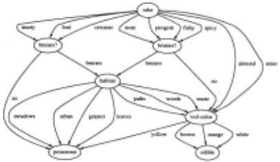
An OODG is an oblivious, read-once decision graph. A constant node is a node such that all edges emanat ing from it terminate at the same node of the subsequent level. Figure 2 shows an OODG derived by the EODG algorithm for the mushroom problem (a post-processing algorithm removes constant nodes to make the graphs more readable) .
OODGs have many interesting properties. These in clude: an OODG for nominal features is canonical for any total function if an ordering on the features is given; any symmetric Boolean function (e.g., parity, majority, and m of n) can be represented by an OODG of size O(n 2 ) ; and the width of levels in OODGs is bounded by min { 2; , k 2 <n-q} for Boolean inputs. We refer the reader to Kohavi (1994a) for a more detailed description of these properties.
3 The EODG algorithm
The EODG algorithm has three phases: growing an oblivious decision tree (ODT), pruning complete levels from the bottom, and merging nodes from the top down. We now describe the phases in detail.
3.1 Top-down Construction Using Mutual Information .
The top-down construction of the 0 DT is performed using mutual information in a manner similar to c4.5 (Quinlan 1993). The main difference is that instead of doing recursive partitioning, i.e., finding a split and con structing the subtree recursively, an iterative process is used.
The general mechanism for growing ODTs is simple: decide on a test with k outcomes that will be done at all nodes in the current level of the tree. Partition the instances at each node p according to the test, and create a new level containing k nodes for each node p in the current level. The k nodes are connected from the parent node p to the k children by edges labelled with the k possible outcomes. Figure 2 shows this algorithm.
The find_split routine determines which split to con duct at all the nodes at the current level, and decides when to terminate. While the test can be of any type, our implementation uses multi-way splits on nominal fea tures (the test outcome is the feature value) and thresh old splits on continuous feature. To determine which
Input: a set T of labelled instances.
Output: an oblivious decision tree for classifying instances. Each set created by tills algorithm has a corresponding node in the graph.
- S = {T} I I S is a set of sets of instances I I t is a test with k outcomes to conduct at all nodes I I in tills level. find_split returns empty-split
- Split s into k sets according to the test t and
- For each of the k sets, create a node and connect to the node representing s. Label edge by the test outcome.
- I I to terminate 2. willle (t = find_split(S)) { 3. S' = {} 4. foreach s E S { add the sets to S'. 7. } I I end foreach 8. S= S'
- } I I end willle
Figure 2: The algorithm for growing the oblivious deci sion trees
feature to split on, and what threshold to pick for con tinuous features, we use mutual information. Our no tation follows that of Cover & Thomas (1991). The conditional entropy H(Y I X1 , 00., Xt) of the label Y given features X 1 , X 2, ... , Xt represents the amount of information about Y after we have seen the values of xl' x2, 0 0 0 'x, and is defined as
Given a new feature X, we define the mutual informa tion as the difference in the conditional entropies:
If£ is zero, the mutual information is defined as
Because the mutual information is biased in favor of tests with many outcomes, we define the adjusted mu tual information as the mutual information divided by log k, where k is the number of outcomes for X. GivenS, a set of sets of instances (each set of instances is a node in the graph), find_split checks all the possible features and determines the one that has the highest adjusted mutual information. For continuous features, we try all possi ble thresholds between two adjacent values of a feature. Computing the best threshold split after the values for a given feature have been sorted can be done in linear time in the number of instances by shifting instances from the left child node to the right child node as the threshold is increased. The technique is exactly the same as that used in Breiman et al. (1984) and Quinlan (1993), except that we determine one split for all the nodes at a level and shift instances from the left child to the right child for all nodes at the current level.
When building a decision tree, it is clear that one should not split on a nominal feature twice, since no information can be gained. However, a surprising phe nomenon that occurs in OODGs, which has no equiva lent in decision tree induction, is that it may be useful to split pure nodes, i.e., nodes that contain instances of only one class, because the merge process may benefit. For example, if we are left with one instance per node, then all nodes are trivially pure. If we split on a relevant feature, some instances will go left and some instances will go right. These nodes will then be merged, and the correct target concept might be identified.
3.2 Merging Nodes
The main advantage of building 0 DTs over regular deci sion trees is that nodes at the same level can be merged because they contain the same test. We begin by de scribing how to convert an ODT into an OODG. We then describe how this merging can be used to conduct top-down pruning, a technique that we believe is more robust to noise than bottom-up pruning and also aids in overcoming splits on irrelevant features by merging the children to a single node as in Figure 2.
Two subtrees in a decision tree are isomorphic if they are both leaves labelled with the same class, or if the root nodes contain the same test and the corresponding children, reached by following the edges with the same labels on both subtrees, are the roots of isomorphic sub trees. Two isomorphic subtrees may be merged without changing the classification behavior of the decision struc ture. While subtree isomorphism may be performed for decision trees too, it is unlikely that subtrees will be iso morphic without the leveling restriction.
The merging process is a post-processing step that is executed after the ODT has been grown. For each level, we check all pairs of nodes for isomorphism, and merge those that are isomorphic. The complexity of the merge process is dominant in the induction of OODGs. At each level with k nodes, O(k 2 ) isomorphic tests have to be conducted. However, because of the kite theorem (Ko havi 1994a), there is a limit on the number of nodes that may be at lower levels, and many merges must succeed at higher levels where the number of nodes is much less than the number of leaves of the ODT.
One advantage of merging nodes comes from the abil ity to assign classes to nodes with no instances. If a split is done and no instances fall to one of the children, the child is labelled with the majority class of the parent.
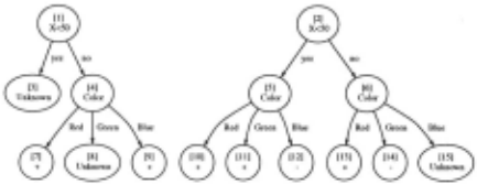
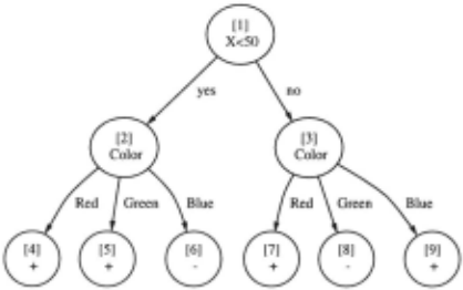
When building the ODT, we leave the node labelled as "unknown" until the merge phase is done, because the merge phase may assign it a class. Intuitively, we would like an unknown node to match anything when we check whether two subtrees can be merged. Two subtrees are defined as compatible if either at least one root is la belled "unknown" (in which case it is a leaf), or if the root nodes make the same test and the corresponding children are the roots of compatible subtrees . Figures 3 shows two compatible subtrees, and Figure 4 shows the merged subtree.
The merging of compatible subtrees changes the bias of the algorithm by assuming that a child node that is marked "unknown" is likely to behave the same as an other child if they belong to compatible subtrees. In order to strengthen the usefulness of the merging pro cess, we split all the nodes at a level that are not leaves labelled "unknown," even those that are pure. Node 4 in Figure 3 is pure, but it has no instances that have the color green. If the node is merged with node 6, it will correctly classify all instances in the training set, but will classify instances that reach the node and have the color green the same way that node 6 classifies them.
In noisy situations, it may be that two subtrees are almost compatible and should be merged, but the above definition of compatibility will not do so. Two subtrees are k-compatible if when we merge them, the number of newly misclassified instances (i.e., instances correctly classified by the subtrees but not by the merged tree) is Input: A training set and a test for each level of the oblivious decision tree.
Output: An oblivious read-once decision graph.
- I I The bottom-up pruning of levels
- Foreach i from 1 to no. levels in full-grown tree do
- ace; = cross-validation ace. of tree grown to level i.
- Let e be the level for which ace; was the highest.
- Let ODT be the oblivious tree grown to level e.
- I I Top-down merging of ODT
- Foreach i from 1 to e {
- Repeat
- For level i, find a pair of nodes that are approx. compatible and merge them.
- } I I End foreach
Figure 5: The bottom-up pruning and top-down merg ing/pruning
less than k. Compatible subtree are 0-compatible. When two nodes are considered for merging, we allow them to misclassify k instances, where k is defined similarly to the pruning method used in C4.5 (Quinlan 1993): the number of misclassifications of each subtree is increased to the high-value of a confidence interval, and the merge takes place only if a similar increase in the merged sub graph results in fewer misclassifications than the sum of the adjusted misclassifications of the children. We have used a 90% confidence interval.
3.3 Bottom-up Pruning
Intuitively, the test for merging nodes checks whether the reduced error-rate due to the nodes being separate is sig nificant statistically. The merging of k-compatible nodes works well in noisy situations only if the misclassification rates at the leaves are non-zero. If the tree overfits the data and has a resubstitution error rate near zero, any merging of subtrees at the top will seem to introduce many misclassifications that are unlikely to happen in a random sample with a large number of instances.
In order to get a more "honest" estimate of the mis classification error at the leaves , we use cross-validation to decide how many levels of the ODT to prune. We fix the order of tests (and thresholds) at the levels, and cross validate every level to get an accuracy estimate. Building an ODT given an ordering is an extremely fast process, so cross-validating the tree at different levels is not an ex pensive process. Note however that the estimate is likely to be slightly optimistic because the split tests were de termined using all the data. Figure 5 shows the bottom up prunmg algorithm and the top-down merge/prune phase.
| Dataset | train | test | features | no | |
|---|---|---|---|---|---|
| SIZe | SIZe | continuous | nominal | classes | |
| australian. all | 690 | 10-CV | 6 | 8 | 2 |
| balance-scale.all | 625 | 10-CV | 4 | 0 | 3 |
| breast.all | 683 | 10-CV | 10 | 0 | 2 |
| chess.all | 3196 | 10-CV | 0 | 36 | 2 |
| cleve.all | 296 | 10-CV | 6 | 7 | 2 |
| crx.all | 653 | 10-CV | 6 | 9 | 2 |
| diabetes.all | 768 | 10-CV | 8 | 0 | 2 |
| flare.all | 1066 | 10-CV | 2 | 8 | 2 |
| german.all | 1000 | 10-CV | 24 | 0 | 2 |
| mushroom.all | 5644 | 10-CV | 0 | 22 | 2 |
| segment.all | 2310 | 10-CV | 19 | 0 | 7 |
| soybean-large. all | 562 | 10-CV | 0 | 35 | 19 |
| tic- tac-toe. all | 958 | 10-CV | 0 | 9 | 2 |
| vehicle.all | 846 | 10-CV | 18 | 0 | 4 |
| vote | 301 | 10-CV | 0 | 16 | 2 |
| monk1 | 124 | 432 | 0 | 6 | 2 |
| monk2 | 169 | 432 | 0 | 6 | 2 |
| monk2-local | 169 | 432 | 0 | 17 | 2 |
| monk3 | 122 | 432 | 0 | 6 | 2 |
| parity5+5 | 100 | 1024 | 0 | 10 | 2 |
| shuttle-small | 3866 | 1934 | 9 | 0 | 7 |
| waveform (21) | 300 | 4700 | 21 | 0 | 3 |
| Dataset | C4.5 | C4.5Rules | EODG | EODT | p-value |
|---|---|---|---|---|---|
| australian.all | 85.36±1.13 | 85.22±1.03 | 82.61±1.85 | 83.19±1.59 | 0.06018 |
| balance-scale.all | 76.94±1.81 | 77.10±2.31 | 86.70±1.22 | 82.20±1.95 | 0.99997 |
| breast.all | 95.32±0.87 | 95.76±0.63 | 95.32±0 .72 | 94.59±0.69 | 0.49119 |
| chess.all | 99.50±0.13 | 99.47±0 .12 | 98.50±0.25 | 98.75±0.22 | 0.00251 |
| cleve.all | 74.98±2.53 | 76.33±3.54 | 78.76±2.54 | 76 .71±2 .88 | 0.86370 |
| crx.all | 84.08±1.08 | 83.93±1.27 | 84.24±1.29 | 85.31±1.16 | 0.54261 |
| diabetes.all | 71.75±1.02 | 72.40±0.95 | 74.74±1.23 | 74.61±1.55 | 0.95714 |
| flare.all | 82.36±1.35 | 81.80±1.22 | 82.64±1.41 | 82.83±1.35 | 0.71643 |
| german.all | 72.50±1.41 | 73.40±1.31 | 70.70±1.78 | 71.40±1.87 | 0.16188 |
| mushroom.all | 100.0±0 .00 | 100.0±0.00 | 100.0±0.00 | 100.0±0 .00 | 0.50000 |
| segment.all | 96.36±0.33 | 96.10±0.45 | 94.76±0.53 | 96.45±0.42 | 0.00321 |
| soybean-large.all | 92.54±1.43 | 91.28±1.00 | 81.13±1.87 | 83.29±1.79 | 0.00002 |
| tic-tac-toe.all | 85.59±1.08 | 98 .85±0 .57 | 89.35±0.96 | 83.20±1.43 | 0.99748 |
| vehicle.all | 69.84±1.77 | 71.86±1.56 | 54.61±2.72 | 66.78±1.02 | 0.00027 |
| vote | 95 .64±0 .52 | 95.87±0.45 | 94.94±0.31 | 94.49±0.61 | 0.08810 |
| monk1 | 75 .70±2.06 | 100.0±0 .00 | 100.0±0.00 | 97.22±0.79 | 1.00000 |
| monk2 | 65.00±2.29 | 65.28±2.29 | 68.52±2 .23 | 68.75±2.23 | 0.82534 |
| monk2-local | 70.40±2.20 | 65.74±2.29 | 98.84±0 .50 | 95.60±0 .98 | 1.00000 |
| monk3 | 97.20±0.79 | 96.30±0.91 | 97.22±0.79 | 97.22±0.79 | 0.50712 |
| parity5+5 | 50.00±1.56 | 50.00±1.56 | 50.00±1.56 | 50.00±1.56 | 0.50000 |
| shuttle-small | 99 .50±0.16 | 99.64±0.14 | 99.74±0.11 | 99.74±0.11 | 0.89174 |
| waveform (21) | 70.40±0.66 | 72.60±0.65 | 65.77±0.69 | 67.13±0.68 | 0.00000 |
| Dataset | C4.5 | EODG | EODT | EODG time in seconds |
|---|---|---|---|---|
| australian | 58.6 | 25.7 | 804.8 | 148.8 |
| balance-scale | 80.0 | 35.5 | 1533.8 | 67.5 |
| breast | 20.4 | 14.7 | 279.2 | 29.9 |
| chess | 56.2 | 69.4 | 14335.0 | 2019.7 |
| cleve | 45 .0 | 12.9 | 152.9 | 32.1 |
| crx | 57.7 | 25.3 | 764.7 | 133.7 |
| diabetes | 122.8 | 18.0 | 319 | 142.6 |
| flare | 2.8 | 4.6 | 26.6 | 151.2 |
| german | 158.4 | 17.2 | 292.6 | 192.5 |
| mushroom | 30 .5 | 31.6 | 329 | 226.4 |
| segment | 81.8 | 179.1 | 6694.4 | 482.9 |
| soy bean-large | 66.5 | 80.9 | 763.1 | 278.7 |
| tic-tac-toe | 129.1 | 64.6 | 2018.2 | 99.0 |
| vehicle | 178.6 | 252.3 | 10209.6 | 574.1 |
| vote | 15.1 | 7.0 | 223.9 | 38.4 |
| monk1 | 18.0 | 7.0 | 53.0 | 3.6 |
| monk2 | 31.0 | 21.0 | 214.0 | 14.3 |
| monk2-local | 47.0 | 16.0 | 125.0 | 14.2 |
| monk3 | 12.0 | 4.0 | 16.0 | 4.0 |
| parity5+5 | 23.0 | 11.0 | 63.0 | 17.8 |
| shuttle-small | 17.0 | 14.0 | 45.0 | 103.0 |
| waveform (21) | 51.0 | 30.0 | 317.0 | 53.8 |
4 Experiments
To estimate the performance accuracy of EODG, we chose a few artificial datasets and real-world datasets from the UC Irvine repository (Murphy & Aha 1994) . The artificial datasets are standard benchmark datasets such as the monk problems (Thrun etal. 1991); from the real-world domains, we chose ones that had at least 200 instances. Because we have not implemented classifica tion of instances with unknown values, we removed all such instances from the datasets tested. Table 1 shows the characteristics of the different domains used. For the artificial domains and for shuttle, we ran a train/test-set sequence. For the other domains, we did 10-fold cross validation.
Table 2 shows the accuracies of C4.5, C4.5-rules, EODG, and EODT (the first two stages of EODG). The last column is the p-value for a paired t-test on the cross validation folds of C4.5 and EODG. (For the runs on a single test-set, we did an unpaired t-test using the sum of the estimated standard deviations from the test set.) For the single runs, we did an unpaired t-test. Values greater than 0.5 indicate that EODG is better and val ues less than 0.5 indicate that C4.5 is better. On many datasets, the behavior of C4.5 and EODG is similar, there are datasets for which EODG's accuracy is worse then C4.5 (soybean-large, vehicle, waveform) , and there are datasets for which the accuracy is better (balance scale, cleve, tic-tac-toe, monk1, monk2-local). It is inter esting to note that on some problems EODT performs better, indicating that the symmetry bias assumed in the merge phase of EODG is not appropriate, but the oblivious restriction does not hurt much.
One of the main advantages of EODG is the small graphs it produces compared to C4.5. Table 3 shows the average sizes for the graphs created for each dataset. EODG clearly creates smaller graphs and when it creates significantly larger graphs (soybean, vehicle) it is also a worse performer. The graphs created by EODT are huge.
5 Future Work
The bottom-up pruning phase of EODG prunes the ODT, which may be inappropriate. For example, parity is badly represented as a tree, and thus the pruning stage reduces the number of features too much. Initial exper iments that involve pruning after merging showed that it may be better (e.g., parity5+5 gives 100% accuracy), but the algorithm becomes too expensive.
The EODG algorithm can be improved along a few directions. We have not implemented handling of un known values, but we believe that an approach similar to that used in decision trees (Quinlan 1993) should work well . We are currently conducting tests on a single feature at a node; other tests, such as oblique splits are possible. Because EODG suffers less from lack of in stances at lower levels, using such tests might not suffer from the same problems that have occurred in decision trees. The disadvantage of such an extension is the loss of comprehensibility that is one of the most important characteristics of decision t rees and graphs over other hypothesis spaces.
We noticed that for continuous features , many splits are made on different thresholds. Since we only merge nodes at the same level, we might consider multi-way splits on real features, as suggested in Fayyad & Irani (1993).
A different approach to feature selection and ordering, which is more feasible in OODGs then in decision trees, is to try different orderings on the features. An ODT on a dataset is defined by a set of tests, one per level, and hence the space of possibilities is much smaller than that of decision trees (although still very large) .
6 Summary
We reviewed the characteristics of oblivious read-once decision graphs as the underlying hypothesis space for in duction algorithms. We introduced EODG, a top-down algorithm that constructs oblivious decision trees using information gain as a splitting criteria and then merges nodes to form oblivious read-once decision graphs. The merging of nodes from the top provides a new way of pruning nodes; in some observed cases, this corrects a split on an irrelevant feature by merging the children.
OODGs have a different bias from that of decision trees, and thus some concepts that are hard to represent as trees are easy to represent as OODGs, and vice-versa (independent of the specific induction algorithm used) . We have shown that for some real-world datasets at UC Irvine, the bias of EODG is appropriate, and for the problems where performance is approximately the same as that of C4.5, EODG produces much smaller graphs.
Acknowledgments
Acknowledgments The work in this paper was done using the M.CC++ library, partly funded by ONR grant N00014-94-1-0448 and NSF grants IRI-9116399 and IRI9411306. We thank Scott Benson and the anonymous reviewers for comments on the paper. We thank Yael Kleefeld and Ya-Huei Wang for their support.
@inproceedings{ijcai1995p139,
  title     = {Oblivious Decision Trees, Graphs, and Top-Down Pruning},
  author    = {Kohavi, Ron and Li, Chia-Hsin},
  booktitle = {Proceedings of the Fourteenth International Joint Conference on
               Artificial Intelligence, {IJCAI-95}},
  publisher = {International Joint Conferences on Artificial Intelligence},
  editor    = {Chris S. Mellish},
  pages     = {1071--1078},
  year      = {1995},
  note      = {Learning},
  url       = {https://ijcai.org/proceedings/1995/139},
}
TY - CPAPER TI - Oblivious Decision Trees, Graphs, and Top-Down Pruning AU - Kohavi, Ron AU - Li, Chia-Hsin T2 - Proceedings of the Fourteenth International Joint Conference on Artificial Intelligence, IJCAI-95 PB - International Joint Conferences on Artificial Intelligence PY - 1995 SP - 1071 EP - 1078 UR - https://ijcai.org/proceedings/1995/139 ER -Copied
Machine-readable versions of this paper, for tools and AI agents:





