
Proposing Measurements in Dynamic Systems
Proceedings of the Fourteenth International Joint Conference on Artificial Intelligence. Knowledge Base Technology. Pages 784-789.
© 1995 International Joint Conferences on Artificial Intelligence
Abstract
Proposing measurements in diagnosis systems for static systems is a well understood task. Usually, entropy based approaches are used, sometimes extended by cost and other considerations. How to do the same task in dynamic systems is less clear, and so far measurement proposal algorithms have been ignored in the recent approaches advanced for dynamic systems. In this paper we will describe a set of techniques and algorithms suitable for measurement proposal in a temporal diagnosis formalism discussed in our previous work . This formalism is based on qualitative Allen constraints. The current paper introduces a measurement proposal algorithm and improves it in several ways. Finally an entropy-based computation method is described for this temporal setting.
- [Allen, 1983] James F. Allen. Maintaining knowledge about temporal intervals. Communications of the ACM, 26(11) :832 -843, 1983.
- [Console et al., 1992] Luca Console, Luigi Portinale, Daniele Theseider Dupre, and Pietro Torasso. Diag- nostic reasoning across different time points. In Pro- ceedings of the 1Oth European Conference on Artificial Intelligence, pages 369-373, Vienna, Austria, 1992.
- [de Kleer and Williams, 1987] Johan de Kleer and Brian C. Williams. Diagnosing multiple faults. Artificial Intelligence, 32:97-130, 1987.
- [Dousson et al., 1993] Christophe Dousson, Paul Ga- borit, and Malik Ghallab. Situation recognition: Rep- resentation and algorithms. In Proceedings of the In- ternational Joint Conference on Artificial Intelligence, pages 166-172 , Chambery, France, August 1993. IJCAI
- [Gamper and Nejdl, 1994] Johann Gamper and Wolf- gang Nejdl. Proposing measurements in dynamic sys- tems. In Working papers of the DX-94 workshop, pages 114-120, New Paltz, NY, October 1994.
- [Mcllraith, 1994] Sheila Mcllraith. Generating test us- ing abduction. In Proceedings of the 4th International Conference on Principles of Knowledge Representa- tion and Reasoning, pages 449-460, Bonn, Germany, May 1994.
- [Nejdl and Gamper, 1994] Wolfgang Nejdl and Johann Gamper. Harnessing the power of temporal abstrac- tions in modelbased diagnosis of dynamic systems. In Proceedings of the 11th European Conference on Ar- tificial Intelligence, pages 667-671, Amsterdam, The Netherlands, August 1994.
- John Wiley & Sons. [Nokel, 1989] Klaus Nokel. Temporal matching: Rec- ognizing dynamic situations from discrete measure- ments. In Proceedings of the International Joint Con- ference on Artificial Intelligence, pages 1255-1260, Detroit, Michigan USA, August 1989. IJCAI
- [van Beek, 1992] Peter van Beek. Reasoning about qual- itative temporal information. Artificial Intelligence, 58:297-326, 1992.
References were extracted automatically from the PDF and may contain errors.
Full text extracted automatically from the PDF; figures, tables and equations may differ. The PDF is the version of record.
1 Introduction
Most current diagnosis systems are able to propose use ful/optimal measurements to discriminate among com peting hypotheses. Several methods have been proposed, mainly based on entropy computations as described in [de Kleer and Williams, 1987]. Recently, some systems for diagnosis of dynamic systems have been proJ,?osed [Console et al., 1992; Nejdl and Gamper, 1994]. lCon sole et al., 1992] is based on a time-slice approach, which considers the system dynamics as a sequence of static states. While this approach restricts expressiveness, it allows to use the same measurement proposal algorithms as in static systems. On the other hand, these static al gorithms are insufficient to be applied in the more gen eral approach described in [Nejdl and Gamper, 1994] . In [Gamper and Nejdl, 1994] we discussed first results on how to propose measurements in our diagnosis system, and this paper extends these results by proposing a set of techniques which propose measurements able to dis tinguish hypotheses described by qualitative temporal constraints.
In section 2 we summarize our diagnostic approach described in [Nejdl and Gamper, 1994] . Section 3 ex plains the concept of measurement proposals and dis-
Wolfgang Nejdl
Universitat Hannover Rechnergestiitzte Wissensverarbeitung Lange Laube 3 30159 Hannover, Germany
cusses the general techniques used to incorporate mea surements into temporal networks. We improve these techniques in section 4 by exploiting the concept of tem poral difference and in section 5 by using the concept of predicted patterns. Section 6 generalizes the entropy computation framework in [de Kleer and Williams, 1987] for our approach. Section 7 discusses related work.
2 Example and Basic Framework
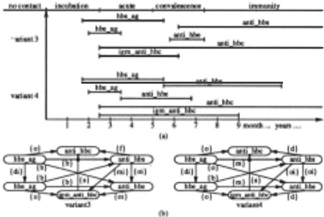
Example 1 (Diagnosis of hepatitis B) In routine test ing of hepatitis B the findings hbs_ag, anti_hbs, hbe_ag, anti_hbe, anti_hbc and igm_anti_hbc are tested, where each of them can assume the value positive (p) or neg ative ( n). A hepatitis B virus infection is characterized by a typical sequence of these findings: 4 acute vari ants (two of them are shown in figure 1a where lines denote the periods of positive findings), and 4 persisting variants. In this paper we do not consider the different stages, e.g. incubation .
All variants look similar, involving basically the same findings. What distinguishes these variants is the order in which these findings occur. In [Nejdl and Gamper, 1994] we described a diagnosis framework which uses a subset of Aliens interval algebra to explicitly represent such temporal relationships.
Temporal Framework. A well known framework to represent qualitative temporal information is Aliens In terval Algebra IA [Allen, 1983], which is based on 13 basic mutually exclusive relations between two intervals: before , meets, overlaps, starts, during, finishes, their in verses and equal, abbreviated as I= {b, m, o, d, s, f, bi, mi , oi, di, si, fi, e} . Indefinite knowledge is expressed as disjunction of basic relations and represented as a set, e.g. (A before B) V (A meets B) is represented as A{b, m}B. We use a graphical representation for a set R of assertions in lA, called !A-network and denoted by n. The nodes represent intervals and the directed arcs are labeled with the relation between the connected in tervals. A missing arc is implicitly labeled with I (no knowledge). Given an !A-network, finding a consistent scenario and finding all feasible relations are basic tem poral reasoning tasks. A consistent scenario is a labeling of the lA-network, where every label consists of a single basic relation and it is possible to map the nodes to a time line such that these relations hold. A basic relation is feasible iff there exists a consistent scenario containing this relation (for more details see [van Beek, 1992]).
Qualitative Temporal Behavior in a Diagnosis Framework. In [Nejdl and Gamper, 1994] we de scribed a model-based framework for diagnosing dy namic systems by explicitly representing qualitative tem poral information a la Allen. Given a system with com ponents COMPS each component has associated a set of behavioral modes. The temporal behavior of each mode is described by a set B of !A-relations between manifes tations assuming that B contains only the feasible rela tions. A manifestation m(v, t) denotes the fact that the parameter m assumes the value v over time interval t. This allows to represent the consequences of a behavioral mode as a complex pattern of temporally overlapping manifestations. The temporal behavior B can be rep resented as an !A-network B. The nodes represent the manifestations, the arcs are labeled with the !A-relation between the connected manifestations. Figure 1 b shows the network representation of the temporal behavior for variant3 and variant4 of hepatitis B. For clarity not all relations are shown. In the diagnostic process we gener ate an abductive and/or consistency-based explanation in terms of behavioral mode assumptions for a set of observations at arbitrary time points and the temporal relations between these observations. Usually, several explanations exists, and to distinguish between them we take additional measurements and continue the diagno sis process. As measurements produce costs we want to perform as few measurements as possible.
In this paper we will discuss how to propose measure ments in our temporal diagnosis framework using the consistency based approach. We will refer to a set HYP of competing explanations as hypotheses h;. We focus on their qualitative temporal behavior B;, except when de scribing how quantitative constraints can improve mea surement proposals. Each parameter has a finite set of possible values. All of them might be used in the descrip tion of the temporal behavior and a parameter assuming the same value might occur more than once.
3 Measurements in Temporal Networks
As dynamic systems are characterized by a complex pat tern of manifestations over long time periods one might expect that measurements should be made in a similar way in a specific order at different times.
Definition 1 (Measurement Proposal) A Measurement Proposal is defined as a formula M 1\ C, where M is a conjunction of expressions m(V, t) suggesting to measure parameter m at timet, and C is a conjunction of qual itative and quantitative temporal relations constraining time t of the measurements.
A measurement proposal is a suggestion to perform the measurements in M in the temporal order indicated by the relations in C. The above definition is very gen eral including measurements at time points and measure ments over time intervals. The relations in C allow to specify the (possibly indefinite) temporal order in which the measurements should be performed, to constrain the measurements relative to the real time line as well as to constrain the duration of measurements . In particular measurements over time intervals are important in do mains like medicine, e.g. did you have headache for at least two hours.
Performing a measurement proposal M 1\ C results in an instantiation of the variables V to the value actually observed, which we call the Outcome 0 of a measure ment proposal.
Example 2 The measurement proposal hbsag(V1 , t1) 1\ hbe_ag(V2, t2) 1\ hbs_ag(V3, t3) 1\ t1 < t2 1\ t2 < t3 sug gests to measure first hbs_ag, after some time hbe_ag, and later again hbs_ag. One of the 8 possible outcomes of this measurement proposal is hbsag(p, tl) 1\ hbeag(p, t2) 1\ hbs_ag(p, t3) 1\ t1 < t2 1\ t2 < t3. Another example is hbs_ag(Vl, t1) 1\ hbeag(V2, t2) 1\ t1 = t2 suggesting to measure hbs_ag and hbe_ag at the same time point with 4 possible outcomes, e.g. hbs_ag(p, tl) 1\ hbe_ag(n, t2) 1\ t1 = t2 . The measurement proposal hbs_ag(V, t) 1\ t = 2 suggests to measure hbs_ag at time 2.
In this paper we only consider measurements per formed at time points and restrict the relations in C to the basic relations { <, =, >} between two time points. In particular, we do not consider quantitative information except for a short discussion on how to improve measure ment proposals by exploiting quantitative constraints. For clarity we will leave out the constraints C in mea surement proposals and their outcomes, use the same time parameter for all measurements related by "=" and assume t; < t i if i < j. If a measurement proposal contains only concurrent measurements we leave out the time parameter as well. Then the first measurement pro posal in the above example and its outcome are repre sented as hbs_ag(Vl, tl) 1\ hbe_ag(V2, t2) 1\ hbs_ag(V3, t3) and hbs_ag(p , tl) 1\ hbeag(p, t2) 1\ hbs_ag(p, t3) respec tively, the second one as hbs_ag(Vl) 1\ hbe_ag(V2) and the outcome as hbs_ag(p) 1\ hbe_ag(n) .
Depending on the outcome of a measurement proposal some hypotheses remain consistent and some other hy potheses are refuted. The aim of a measurement pro posal algorithm in a diagnosis system is to find proposals which reduce the hypothesis space.
3.1 A Measurement Proposal Algorithm
We have to find a measurement proposal with a possi ble outcome which supports one hypothesis and refutes another one. The outcome of a measurement proposal supports a hypothesis if we can fit each observed value into the temporal behavior of the hypothesis and the temporal relations of the measurement proposal are sat isfied; otherwise, the hypothesis is refuted. As we do not have time points in our temporal framework we assume that the measured value holds over a small time inter val "around" the measurement time point . It is easy to show that this assumption does not influence the results.
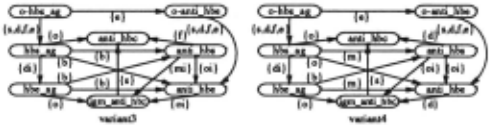
The following procedure MEASPRo implements a measurement proposal strategy. For each hypothesis h; E HYP we maintain a set S; of !A-networks initially containing the corresponding temporal behavior network B;. For each hypothetical measurement with outcome m(v, t) we insert a measurement outcome node anode representing the small time interval around t into each !A-network N in S; and constrain it as follows :
- For each other measurement outcome node anode' at time point t' we add the !A-relation on ode { b} on ode' if t < t', on ode { e} on ode' if t = t' and onode{bi}onode' if t > t'.
- We constrain the anode to occur within a manifes tation node mnode in the temporal behavior repre senting the same parameter m and the same value v by adding the relation on ode { s, d,f, e} mnode. If several such mnodes (same parameter and value) are related by before (after) the on ode can only occur in one of them at a time. In this case we construct for each such mnode a copy of the actual N to represent the different possible constraints of anode .
- We constrain anode to occur outside each mnode representing parameter m and value v' =f. v by adding the relation onode{b, m, bi, mi}mnode.
Finally we test consistency for each IA-network in S; us ing known temporal reasoning algorithms [Allen, 1983; van Beek, 1992] and remove inconsistent networks. Situ ations , where we haveS;, Sj such that S; =f. 0 and Sj = 0 characterize possibly discriminating measurement pro posals for the hypotheses h; and hj.
Example 3 We choose the measurement hbs_ag(Vt , t) with a positive outcome, insert the measurement out come node o-hbs_ag into the !A-networks for variantS and variant4 and constrain it to be within the tem poral extent of hbs_ag, i.e. o-hbs_ag{s, d,f,e}hbs_ag . The positive hbs_ag is consistent with both variants , and we continue with a new hypothetical measure ment at the same time point , e.g. anti_hbe(V2, t) with a positive outcome. Adding o-anti_hbe{ e }o-hbs_ag and o-anti_hbe{ s, d, f, e }anti_hbe (figure 2) and prop agating these relations yields an inconsistency in variantS (due to hbs_ag{ b} anti_hbe ), but it is con sistent in variant4 . Thus the measurement pro posal hbs_ag(V1 , t) A anti_hbe(V2,t) has an outcome hbs_ag(p, t) A anti_hbe(p , t) which can distinguish be tween the two variants.
The algorithm MEASPRO makes no assumptions about whether measurements are proposed in the past or in the future. In some domains measurements in the past make sense, e.g. in the medical domain.
Definition 2 (Confirmation, Refutation) The outcome 0 of a measurement proposal M 1\C confirms hypothesis h iff the lA-network consisting of the temporal behavior B extended by the outcome 0 according to the strategy of algorithm MEASPRO is consistent. Otherwise, the outcome 0 refutes hypothesis h.
Definition 3 (Possibly-Discriminating) A measure ment proposal M 1\ C is Possibly-Discriminating for a set HYP of hypotheses iff it has a possible outcome 0 and there exists h; , hj E HYP such that 0 confirms h; and refutes hj .
This definition ensures that a possibly-discriminating measurement proposal has at least one possible outcome which allows to reduce the hypothesis space.
· Example 4 The measurement proposal hbs_ag(Vt) A hbe_ag(V2) is not a possibly-discriminating one as the temporal relationship between hbs_ag and hbe_ag is { di} in both hypotheses and thus the possible out comes in both hypotheses are the same, i.e. hbs_ag(p) 1\ hbe_ag(n) , hbs_ag(p) 1\ hbe_ag(p) and hbs_ag(n) A hbe_ag(n). Another measurement proposal which is not possibly-discriminating is anti_hbs(Vt) 1\ anti_hbc(V2) although the corresponding relation is {!} in variant3 and { d} in variant4 . Both relationships allow all pos sible outcomes except anti_hbs(p) A anti_hbc(n). An example of a possibly-discriminating measurement pro posal is hbs_ag(Vt) 1\ anti_hbe(V2)· As the temporal re lationship is { b} in variantS and { o} in variant4 the out come hbs_ag(p) 1\ anti_hbe(p) occurs only in variant4 . Another possibly-discriminating measurement proposal is hbs_ag(Vt, tt) 1\ anti_hbs(V2, tt) 1\ hbs_ag(Va , t2) A anti_hbs(V4 , t 2) 1\ hbs_ag(Vs, ta) 1\ anti_hbs(Vs, ta). The outcome hbs_ag(p, tt) 1\ anti_hbs(n, t1) A hbs_ag(n, t2) A anti_hbs(n, t2) A hbs_ag(n, ta) 1\ anti_hbs(p, ta) con firms variantS, which has hbs_ag { b} anti_hbs, and re futes variant4, which has hbs_ag { m} anti_hbs .
MEASPRO represents a very general method but it has some drawbacks. First, implementing a nondetermin istic procedure represents some difficulties, and can be very inefficient if implemented as a simple generate and test procedure. Second, it performs temporal constraint propagation [Allen, 1983; van Beek, 1992] for each hy pothetical measurement, which can be very costly since it depends on the whole network. Moreover, consistency testing in lA is exponential, and we have to use approx imation algorithms which in general are not complete. In the following we will show how we can improve upon our measurement proposal algorithm.
4 Exploiting the Temporal Difference
The generation of measurements can be focused by ex ploiting the difference in the predicted behavior of hy potheses. In the simplest case this can be a parameter predicted only in one hypothesis, which is trivial and thus not considered here. As each hypothesis is charac terized by a typical sequence of temporally overlapped manifestations we will rather focus on the temporal dif ference of hypotheses (assuming that each hypothesis is described by the same parameters).
Definition 4 (Temporal Difference) Given are 2 hy potheses h1 and h2 and their qualitative temporal be havior B1 and B2. The Tempoml Difference between ht and h2 is defined by the two sets of !A-relations
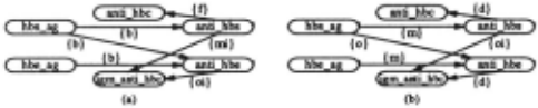
The difference set Dt,2 (D2,1) between ht and h2 con tains those relations which occur only in B1 (B2) but not in B2 (Bt) . For each pair of hypotheses these two sets capture the difference in their temporal behavior. An empty relation R;j = 0 in D1,2 means that R}i ~ Rl-, i.e. all basic relations between m; and mj in h1 are alfowed in h2 . In D 2,1, however, we might still have a nonempty set. The temporal difference D1,2 can be represented as a graph DG1,2, called Tempoml Difference Graph. The nodes represent manifestations, the directed arcs are la beled with the relations in Dt 2· Arcs labeled with the empty set need not be drawn. 'Figure 3 shows the tem poral difference graphs for variantS and variant4.
As the two difference graphs for two hypotheses cap ture all differences in the temporal behavior we use them to focus the generation of measurement proposals. The following proposition helps to reduce the measurements to be considered.
Proposition 1 Given are two hypothesis h1 and h2. A necessary condition for a possibly-discriminating mea surement proposal M 1\ C suggesting to measure mt to mn is that there exist m;, mj such that m; and mj are connected in DG1,2 or DG2,1 ·
Example 5 Let us consider the difference graphs for variant3 and variant4 in figure 3. Applying the above proposition we never propose measurements consisting of a subset of hbs_ag, hbe_ag, igm_anti_hbc and anti_hbc. Indeed, looking at figure 1 we recognize that the quali tative temporal relations between these manifestations do not differ from each other in both variants. For concurrent measurements of two parameters we have to consider only 6 measurement proposals instead of 15 without difference graphs. We have the 3 possibly discriminating measurement proposals hbs_ag(Vt) 1\ anti_hbe(V2), anti_hbs(Vt) 1\ igm_anti_hbc(V2) and anti_hbe(Vt) 1\ igm_anti_hbc(V2). Examples of two con nected manifestations in the difference graphs which do not provide a possibly-discriminating measurement pro posal are hbs_ag(Vt) 1\ anti_hbs(V2) and anti_hbs(Vt) 1\ anti_hbc(V2)· However, these parameters provide possibly-discriminating measurement proposals if mea sured 3 times as we have seen in the last example for hbs_ag and anti_hbs.
Temporal difference graphs tell us more. Suppose we can only perform measurements at the current time point and in the future. The temporal difference graph can be used to avoid measurements which only would provide discriminating information if performed in the past. For instance, if we measured anti_hbe to be positive then it makes no sense to measure hbe_ag at the current time point or in the future. The relation between hbe_ag and anti_hbe is { b} and { m} in the corresponding difference graphs indicating that the temporal extent of hbe_ag al ready terminated. Another example is when the differ ence graphs contain mt { s }m2 and m1 { o }m2. If we mea sure m2 to be positive then measuring m1 at the same time or later provides no discriminating information.
5 Predicted Patterns
Difference graphs give us a means to reduce the num ber of measurement proposals which have to be consid ered as possibly-discriminating. However, the test for possibly-discriminating itself still has to be done using constraint propagation on temporal networks. To avoid this second source of complexity, we introduce the con cept of predicted pattern tables, which basically compile the result of testing measurement proposals for consis tency. The basic idea we use is that temporal relations can be characterized by predicted patterns. For the sake of simplicity we introduce an alternative representation for measurement proposals and their outcomes. As we allow only the basic point relations the manifestations in a measurement proposal can be partially ordered.
Definition 5 (Measurement Tuple/Sequence) A Mea surement Proposal M 1\ C can be represented as a Measurement Sequence mts = « mtt(tt), ... , mtn(tn) », where t; < tj for i < j. Each mt; is called a Measure ment Tuple mt(t) = (m1, ... , mn) and is a suggestion to measure the parameters m; at time point t .
Definition 6 (Pattern/Pattern Sequence) The outcome of a measurement tuple mt(t)=(mt, .. . , mn) is called a Measurement Pattern mp(t)=(v1, ... , vn), where each v; is a possible outcome for parameter m;. The out come of a measurement sequence is a sequence of mea surement patterns mps = « mp 1 (tt), ... , mpn(tn) », called a Measurement Pattern Sequence .
We will leave out the time parameter in measurement tuples and patterns. Measurement sequences suggest ing to measure the same tuple mt n times are abbre viated as (mt)n. For instance, the measurement pro posal hbs_ag(Vt, tt) 1\ anti_hbe(V2, tt) 1\ hbs_ag(V3, t2)
| Ba.sic rei. | Meaning Predicted pattern sequence | |||||
|---|---|---|---|---|---|---|
| z before y x meets y z overlaps y x starts y z during 11 z finishes y z equal y | "' ..!... - - - - - | (x,'Y) (x,'Y) (x,'Y) (x,'Y) (X,y) ~:~~ ,!/ | (z,y) (z,y) (z,y) (x,y) (X,y) | (x,'Y) (z,y) (z,y) (z,y) ~~· ~~ z,y | (x, y) (x,y) (x,y) (x,y) (x,y) | ('X,y) (x,'Y) (x,'Y) (X,y) (x,'Y) ~:~~ ,'Y: |
z equal y -
Table 1: !A-relations and predicted pattern sequences.
1\ anti_hbe(V4, t2) can be represented by the measure ment sequence (hbs.ag, anti_hbe) 2 · One possible out come of this measurement sequence is the pattern se quence « (p, n), (p, p) ».
5.1 Predicted Pattern Sequences
Obviously, there is a strong relationship between pattern sequences and the qualitative temporal relations in lA. Let us consider the meets-relation between hbs_ag and anti.hbs in variant4 (figure 1). It can be characterized by two consecutive time slices: in the first time slice hbs_ag is positive and anti_hbs is negative and in the second time slice hbs_ag is negative and anti.hbs is positive.
Definition 7 (Predicted Pattern Sequence) Each basic relation in lA is characterized by a specific pattern se quence, called Predicted Pattern Sequence.
Table 1 shows the basic relations (without the inverse relations) in lA and their predicted pattern sequences. x and y denote that the property associated with the cor responding interval holds, x and y denote that the corre sponding property does not hold. As the basic relations are mutually exclusive the predicted pattern sequences are too. We therefore get the following proposition:
Proposition 2 Given are two hypothesis h1 and h2 . A sufficient condition for a possibly-discriminating mea surement sequence (m;, mj)n for h1 and h2 is that n 2: 5 and m; and mj are connected in both difference graphs.
It is important that the two parameters are connected in both difference graphs stating that both hypotheses have a unique relation, which can be recognized by a sequence of length 5. If we assume a measurement rate which recognizes each value change of the parameters we can give stronger conditions.
Proposition 3 Given are two hypothesis h1 and h2 and the assumption that each value change of a parame ter is recognized. A sufficient condition for a possibly discriminating measurement sequence (m;, mj )n for h1 and h2 is that n 2: 4 and that m; and mj are connected in at least one of the two difference graphs.
This proposition ensures that whenever two hypothe ses differ in their qualitative temporal behavior there exists a possibly-discriminating measurement sequence suggesting to measure two parameters 4 times. Of course, in some cases even smaller sequences are suffi cient. In the next section we look at sequences of length one, i.e. measurement tuples.
| Relation tuples | Predicted Patterns | |||
|---|---|---|---|---|
| ~b~, \~~~ (bi), (mi) (o), (oz) (s), (d), (f) (si), (di), (fi) (e) | (p,p) (p,p) (p,p) (p,p) | ~p, n~ (p, n) (p, n) | ~n,p~ (n,p) (n,p) | ~n, n~ (n, n) (n, n) (n, n) (n, n) |
5.2 Predicted Pattern Tuples
Sequences of measurements postpone a distinction be tween several hypotheses into the future. Sometimes it is better to choose a measurement consisting of a set of concurrent measurements (even if they are more expen sive) rather than a sequence of measurements.
A set R of !A-relations between n manifestations can be represented by two tuples: a tuple ( m1, ... , mn) of manifestations and a relation tuple R(m 1 , ... ,mn) = (R12, ... , R1n, R23, ... , R2n , ... , R(n-l)n) of length n(n1) /2 corresponding to the number of manifestation pairs. For instance, the relations { hbs_ag(p) {b} anti_hbs(p), hbs_ag(p) {di} hbe_ag(p), hbs_ag(p) {b} anti_hbe(p), anti_hbs(p) {bi} hbe_ag(p), anti_hbs(p) { oi} anti_hbe(p), hbe_ag(p) { b} anti_hbe(p)}, between the positive hbs_ag, anti_hbs, hbe.ag and anti_hbe in vari ant:Jcan be represented by m = (hbs_ag(p), anti_hbs(p), hbe_ag(p ), anti_hbe(p )) and Rm = (b, di, b, bi, oi, b).
Definition 8 (Predicted Pattern) Given is a set R of !A-relations between the manifestations m1 , ... , Tnn as suming the values v1, ... , Vn. A pattern pp=(v~, .. :, v~), where each vi is a possible value of m;, is called a Pre dicted Pattern by the relation tuple R(m 1 , ... ,mn) iff the following set of !A-relations is consistent:
The basic idea of this definition is the same as the one used in algorithm MEASPRo. The pattern node is constrained to be within ( { s, d,f, e}) or outside ( {b, m, bi, mi}) the corresponding manifestation nodes. This tells us that the pattern pp appears somewhere in the temporal behavior specified by R. More formally, there is a consistent scenario of R containing a time slice corresponding to the pattern pp.
We use the definition above to generate all relation tu ples which predict a specified pattern (v1, ... , vn)· Given a measurement tuple (m1, ... , mn), we apply this defini tion for each possible pattern (outcome) mp initializing the relations between the m; 's in R to the set I of all basic !A-relations and construct a table with relation tu ples and predicted patterns. Table 2 shows all relation tuples and the predicted patterns for a measurement tu ple oflength 2. In [Gamper and Nejdl, 1994] we describe in more detail how to construct the tables.
Using table 2 to find a measurement of length 2 turns out to be a simple table lookup. A measurement tuple is possibly-discriminating for two hypotheses h1 and h2 iff the corresponding relation tuples from B1 and B2 pre dict different sets of patterns. For disjunctions of basic relations we take the union of the patterns predicted by the basic relations, e.g. for { s, e} we take the union of the patterns predicted by (s) and (e), which is the set of all possible patterns. Again we use the difference graphs to reduce the number of tuples to be considered.
| Rel. tuples | Predicted Patterns |
|---|---|
| ~b, si, bi). | ~p,n,p~ ~n,p,n~ ~n,n,n~ \P, n, n; |
| (o, si, mi) | (p, n,p) (n,p,n) (n,n,n) (p,p, n) |
Example 6 Let us consider the measurement tuple (hbs_ag, anti_hbe) where we have a {b }-relation in vari ant3 and an { o }-relation in variant4. The corresponding relation tuples (b) and (o) predict different sets of pat terns. The pattern (p,p) is only predicted by (o) . Thus, (hbs_ag, anti_hbe) represents a possibly-discriminating measurement tuple. A measurement which is not a possibly-discriminating one is ( anti_hbs, anti_hbc) with the corresponding relations (!) and (d) .
Obviously, if we use only the 2-tuple table, no infer ences are compiled over more than two measurements . If we want to propose a measurement tuple of length 3, the table tells us only about the pairwise c~nsistency of the measurements included in this tuple. If we want to get better discriminating power, we have to construct similar tables for larger tuples of relations and patterns. Table 3 shows a part of the relation tuples and the pre dicted patterns of length 3.
Example 7 In this example we assume that the pos itive hbs_ag and hbe_ag start at the same time, i.e. hbs_ag{si}hbe_ag. The measurement tuple (hbs_ag, anti_hbe) is a possibly-discriminating tuple, as it allows a distinction in the case of (p, p) as seen from table 2. If we look at the measurement tuple (hbs_ag, anti_hbe, hbe_ag) (i.e. adding the additional measurement hbe_ag), we get no additional distinguishing patterns from the 2-tuple table. However, the 3-tuple table gives us an additional distinguishing pattern for the whole 3-tuple measurement, i.e. (p, n, n), which excludes variant4.
Propositiou 4 Given are two hypothesis h1 and h2 with temporal behavior B1 and B2 . A sufficient con dition for a possibly-discriminating measurement tuple (m1, ... , mn) for h1, h2 is that the corresponding relation tuples from B1 , B2 predict different sets of patterns.
Generating the predicted pattern tables requires to find all consistent scenarios for sets ofiA-relations which is in general intractable. However, we can precompile these tables, and the set of relations depends only on the length of the measurement tuples and not on the size of the temporal behavior of the hypotheses as in MEASPRo .
6 Evaluating Measurements by Entropy
So far, we have only checked for possibly-discriminating measurement tuples. What we will do now is to gener alize the entropy computation framework from [de Kleer and Williams, 1987] to our case. We have to use whole measurement tuples instead of single measurements and we have to deal with hypotheses which predict more than one value for a measurement tuple.
Given are a set HYP of hypotheses h; and their tem poral behavior B;. For a measurement sequence mts = (mt 1, ... , mtn) we represent the corresponding relations in B; as relation tuple R!nts and the set of predicted pat tern sequences as P:,.ts· The set of possible pattern se quences of mts is MPS mts· We construct for each pattern sequence mps E MPS mt· the set HYP mps of hypotheses which predict the pattern sequence mps. These sets pro vide the basis of our analysis. Obviously, each hypothesis h; appears in at least one HYP mps. The measurement sequence mts is possibly-discriminating iff there are at least two different sets HYP mps 1 :/= HYP mp· 2 , where at least one of these sets is neither the empty set nor the set of all hypotheses.
Now the expected entropy for the hypothesis proba bilities given a measurement sequence mts is given by
p(mts=mps) is the probability that the outcome of mts is mps and H ( mts= mps) is the entropy of the hypothesis probabilities given the hypothetical measurement result mps. The best measurement sequence mts is the one which minimizes the expected entropy He ( mts) of hy pothesis probabilities [de Kleer and Williams, 1987].
The probability p( mts=mps) is given by the formula p(mts=mps) = "'L.h;EHYP p(mts=mps/h;)p(h;), where p(h;) is the probability that h; is the actual hypothesis, and p(mts=mpsfh;) is the conditional probability that the outcome of mts is mps assuming h; is the actual hy pothesis. In dynamic systems this probability depends on the duration of mps appearing in h;. If we do not have quantitative information concerning the temporal extent of intervals in B; we can use the approximation p(mts=mpsjh;) = "'L-mps'EP; :mpsCmps' ~IP'l I assummt· - mt. ing that each measurement pattern sequence predicted by h; has equal probability ( mps [; mps' means that mps is a subsequence of mps'). Note, that this is a case where using quantitative information really helps.
The entropy H ( mts=mps) of hypothesis probabili ties under the assumption that mts is measured to be mps is given by the formula H(mts=mps) = - "'L.h;EHYP p(h;/mts=mps) logp(h;/mts=mps), where p(h;/ mts=mps) is the probability that h; is the hypoth esis given that mts has been measured to be mps, and can be computed using the Bayes rule.
Example 8 We consider the hypotheses variant3 and variant4 and the measurement tuple (hbs_ag, anti_hbe) with the possible patterns (p, p), (p, n), (n, p) and (n, n). (p, p) is only predicted by variant4 whereas all other patterns are predicted by both variant3 and variant4. In table 4 we summarize the results of calculating the expected entropy. As the pattern (p, p) distinguishes between both hypotheses its entropy is 0. For the other patterns the entropy is 0.98. The overall expected en tropy for the measurement tuple (hbs_ag, anti_hbe) is ap proximately 0.87. For the other possibly-discriminating measurement tuples of length 2 we get the same value, since they also have exactly one measurement pattern which allows to distinguish among the two variants. Hence, all three measurement tuples of length 2 are ex pected to distinguish equally well, if we cannot exploit quantitative information. If we have quantitative infor mation as in figure 1, then the best measurement tu ple would be (anti_hbs, igm_anti_hbc), because the inter val corresponding to the discriminating pattern is larger than for all other measurement tuples.
7 Discussion
Proposing measurements which discriminate between a set of hypotheses is an important issue in diagnostic rea soning. For model-based diagnosis of static systems sev eral algorithms has been developed, mostly variations of the entropy-based algorithm described in [de Kleer and Williams, 1987] . Mcllraith [Mcllraith, 1994] re cently examined the problem of test generation for hypo thetical reasoning in general including diagnosis. While some of the concepts are similar to ours, e.g. a rele vant test in [Mcllraith, 1994] corresponds to a possibly discriminating test in our framework, Mcllraith charac terizes test generation as an abduction problem, while we start with a nondeterministic algorithm and end up with efficient table lookup techniques. The major difference , however, is that we investigate measurement proposal for dynamic system and hence focus on the different tempo ral behavior of the hypotheses.
As far as we know no work has been done in propos ing measurements in reasoning about dynamic systems. Most closely related to our work are situation recogni tion systems. Nokel [Nokel, 1989] describes a system for generating measurement sequences in order to recognize dynamic situations, which also uses a subset of Aliens interval algebra. The main difference to our approach is that we propose measurements to distinguish among several hypotheses characterized by a dynamic behav ior which is different from recognizing such hypotheses . Distinguishing among several behaviors is based on their difference, while recognizing them involves observing all their characteristics. Indeed, Nokel proposes at least one measurement for each manifestation. While Nokel plans sequences of measurements allowing only one measure ment at a single time point and does neither discuss en tropy based algorithms nor efficiency improvements like we do, we investigate concurrent measurements as well as measurement sequences, including entropy based pro posal algorithms and give a set of efficiency improving techniques to check for distinguishing measurement tu ples. Another situation recognition system similar to Nokels approach is described in [Dousson et al. , 1993].
8 Conclusion
In contrast to static model-based diagnosis systems, current model-based formalisms for temporal diagnoses have not yet investigated the issue of proposing mea surements in a dynamic setting. In this paper we in vestigate techniques and algorithms for proposing new measurements in the temporal diagnosis framework de scribed in [Nejdl and Gamper, 1994] which represents explicitly qualitative temporal behavior using a subset of Allen relations. We discuss a general (nondeterministic) algorithm based on constraint propagation for proposing possibly-distinguishing measurements. We show how the efficiency of this method can be improved by using tem poral difference graphs and table lookup in precompiled predicted pattern tables. Finally, we generalize the en tropy based measurement proposal algorithm defined in [de Kleer and Williams, 1987] to our temporal setting.
@inproceedings{ijcai1995p102,
  title     = {Proposing Measurements in Dynamic Systems},
  author    = {Gamper, Johann and Nejdl, Wolfgang},
  booktitle = {Proceedings of the Fourteenth International Joint Conference on
               Artificial Intelligence, {IJCAI-95}},
  publisher = {International Joint Conferences on Artificial Intelligence},
  editor    = {Chris S. Mellish},
  pages     = {784--789},
  year      = {1995},
  note      = {Knowledge Base Technology},
  url       = {https://ijcai.org/proceedings/1995/102},
}
TY - CPAPER TI - Proposing Measurements in Dynamic Systems AU - Gamper, Johann AU - Nejdl, Wolfgang T2 - Proceedings of the Fourteenth International Joint Conference on Artificial Intelligence, IJCAI-95 PB - International Joint Conferences on Artificial Intelligence PY - 1995 SP - 784 EP - 789 UR - https://ijcai.org/proceedings/1995/102 ER -Copied
Machine-readable versions of this paper, for tools and AI agents:





