Second Order Measures for Uncertainty Processing

1 Introduction

Numerical values describing the uncertainty of knowledge and data in knowledge-based (KB) systems are usually imprecise due to t11e fact that they are almost always provided as the subjective assessments of experts or users. Nonetheless, these imprecise numbers are processed by some algoritlun and the results are used to draw conclusions. Without a thorough KB verification which includes an analysis of the robustness of the uncertainty processing technique used, we must always be aware of the limited credibility of results. This paper aims to provide techniques for such an analysis. The methods described are based on compositional (extensional) calculation of uncertainty processing [Duda et al., 1976; Gashnig, 1980; Heckerman, 1986; Reiter, 1980; Wise, 1988] (see [Hajek et al., 1992; Pearl , 1988] for more detailed discussion). Although the current attention of the AI community is focused rather on intensional (model-based, probabilistic) approaches [Spiegelhalter, 1986; Lauritzen and Spiegelhalter, 1988; Pearl, 1988], the compositional methods are still popular due to t11eir computational simplicity. The main objection to the compositional methods is that the results are not sound. In [Hajek et al., 1992] an attempt is made to revive these methods by replacing t11e original simple-minded Let x, y and z be partial certainty factors of a hypothesis.

1. If x = 1 andy :;t: -1, or y = 1 and x :;t: -1 then x ffi y = 1. If x = -1 and y :;t: 1, or y = -1 and x :;t: 1 then x ffi y = -1.
2. If x = 1 andy= -1, or y = 1 and x = -1 then x ffi y is not defmed.

1. For x, y, z :;t: -1 and x, y, z :;t: 1
2. (a) x ffi y = y ffi x ... commutativity
3. (b) (x ffi y) ffi z = x ffi (y ffi z) ... associativity
4. (c) x ffi 0 = x

... null element

• (d) x ffi -x = 0 ... inverse element
• (e) If x :S; y then x ffi z :S; y ffi z ... ordering

These axioms describe the properties we intuitively expect from combining operations. The axioms 3 (a)- (e) define an ordered Abelian group (OAG) over (-1, 1) with the group operation ffi so far unspecified. This OAG is isomorphic with the additive OAG over (-oo, oo); there are various isomorphisms which map -1 ~ -oo, 0 ~ 0, 1 ~ oo, the group operation ffi being the normal addition and the inverse element being the number with the opposite sign. Similarly, the OAG over (-1, 1) is isomorphic with the multiplicative OAG over (0, oo), i.e. -1~0. 0~1. 1 ~ oo , the group operation being the multiplication and the inverse element of x being 1/x. Particular combining operations ffi over (-1, 1) can be defined by means of these isomorphisms. For example, if we use the additive OAG the partial weights x and y to be combined are mapped by some isomorphism from (-1, 1) to (-oo, oo), then the isomorphic images are summed since addition is the group operation on (-00, oo), and finally the result is mapped back by the inverse isomorphism to (-1, 1). The group operation defines a combining function g(x,y):

There are several isomorphisms (-1, I) to (-oo, oo) suggested by [Hajek et al., 1992]. We will mention only two of them: those used in Emycin and Prospector. They are defined for (0, 1) ~ (0, oo) by the following formulae, for negative values we take an odd extension, F(-x) = -F(x).

Substituting (2) to (1) gives Emycin formulae. Similarly, substituting (3) to (1) gives (x + y)/(1 + xy) which is the Prospector odds-based formula recalculated into (-1, 1).

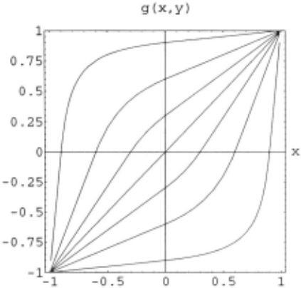
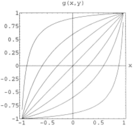
The isomorphisms between Prospector and Emycin were used in [Heckerman, 1986] to interpret MYCIN's certainty factors. Similarly, the AL/X uncertainty processing method [Reiter, 1980] is just an isomorphic image of the Prospec­ tor's. Graphs of combining functions defined by (2) and (3) are shown in Fig. 1 (a) - (b) for y = - 0.9, - 0.6, - 0.3, o.o, 0.3, o.6 and o.9.

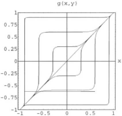
In order to demonstrate that our intuition expressed by axioms 3 (a) - (e) is not sufficient to guarantee sensitivity properties required for processing of uncertain knowledge we have defined the combining function as follows:

We will show this function to be a typical counter­ example which does not meet acceptable sensitivity properties. Its graph is shown in Fig. 1 (c).

3 Sensitivity functions

For applications, the exact values of certainty factors must not be crucial. Uncertainty processing methods must provide correct results regardless of small variations in numerical values. From this point of view we expect the processing methods to be insensitive to small changes. On the other hand the method must "weigh" the contributions; the global certainty factor must depend on the values of partial ones which means that it must not be too insensitive. Given a standard rule-based architecture it is reasonable to assume that no knowledge is represented in terms of the combining method, i.e. we will consider the same, a priori determined, combining function throughout the inference network. The sensitivity of the final hypothesis depends on the sensitivi­ ties of rules and the sensitivities of combining algorithms. The behaviour of the combining function for small varia­ tions of one variable is described by the first partial deriva­ tive with respect to this variable.

Definition 1

The sensitivity function sx(x,y) of a combining function g(x,y) with respect to xis

Similarly we define the sensitivity function with respect toy as sy(x,y) =Jg(x,y)/Jy. Since the operation EB is associative, we can extend the concept of binary combining functions to n-ary ones as follows:

The concept of a sensitivity function can also be extended

The sensitivity functions have the following properties:

Proposition 1

Fora and b E (-1,1), sx(a,b) = sy(b,a), i.e. the sensitivity functions are symmetric.

Proposition 2

sx(a,b) =sx(-a,-b), i.e. the sensitivity functions are even functions of their arguments.

Proposition 3

sx(a,b) ~ 0, i.e. the sensitivity functions are non-negative.

The following two propositions show that n-ary sensitivity functions can be composed of binary ones.

Proposition 5

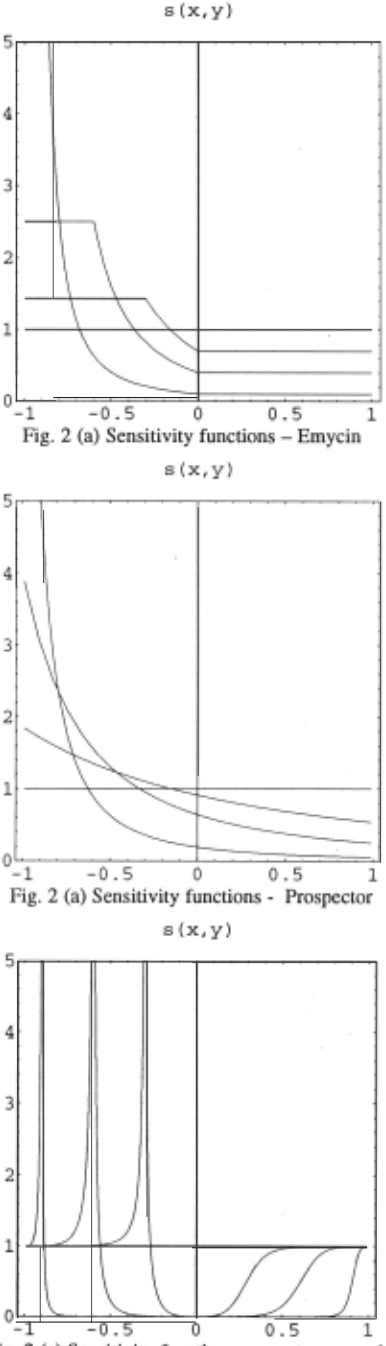
The sensitivity functions corresponding to (2), (3) and (4) are shown in Fig. 2 for y = 0, 0.3, 0.6 and 0.9. The completion for y < 0 describes Proposition 2.

For proofs of all the propositions introduced in this paper see [Zdrahal, 1991a].

What kind of sensitivity function do we prefer? Whereas in control theory the minimum sensitivity with respect to parameter variation is a clear goal, here it is more difficult to define an ideal sensitivity behaviour since we are interested in an input sensitivity. Therefore the answer necessarily is rather speculative.

If both arguments are of the same sign, the sensitivity should be approximately constant. The combining function weighs partial certainty factors. As both arguments approach the same extreme value (+1 or -1) the sensitivity function should go to zero. We are almost certain that the hypothesis holds (for +1) or does not hold (for -1) and small variations do not have any impact. The sensitivity increases as the partial certainty factors are approximately of the same absolute value but with different signs. The partial certainty factors compensate each other and the result is close to zero.

The combining functions of both Emycin and Prospector satisfy our intuitive insight. The required weighing effect prevails. On the contrary, function (4) almost does not weigh at all. Instead, it has a switching character. For some y 0 > 0 and- y0 < x < y0 the impact of xis negligible (see Fig. 2 (c)). The value of x becomes important only near- y 0 = x . At this point the combining function completely switches to the global certainty factor of the opposite sign. The narrow band around- Yo = x is overly sensitive and unstable. In this case sx(x,y) has even got a singularity point at- Yo = x .

Out of interest we have also evaluated the conditional probability P(H I E1, E2) calculated from P(H I E1) and P(H I E2) by means of the maximum entropy criterion [Zdrahal, 1991b]. Both hypothesis Hand evidences E1 and E2 were binary valued, probabilities were recalculated into ( -1,1) and the values were expressed in terms of a "combining function". We are fully aware that this function is based on a completely different (intensional) philosophy: it has nothing to do with axioms 3 (a)- (e), cannot be expanded by (5) and thus it is impossible to carry out a fair comparison. However the corresponding sensitivity function proved to be very similar to that of Emycin and Prospector (Fig. 2 (a) and (b)) and very different from that of Fig. 2 (c).

From a sensitivity point of view, the formulae (2) and (3) on the one hand and (4) on the other hand produce very different types of combining functions. The properties, however, become more obvious if we take into account the fact that all of them must {)bey the following proposition.

Proposition 6

The average value of sensitivity over interval (-1,1) is constant and equals 1, i.e.

This propositiOn in combination with Proposition 3 implies that an excessive sensitivity of the combining function on some subintet"val must be compensated by insensitivity in some other subinterval. This effect can be observed in Fig. 2. In cases (a) and (b) there is an even sensitivity on the major part of the certainty interv-al. On the contrary, in case (c) there is extreme sensitivity around the switching point which is necessarily compensated by almost zero sensitivity in a large subinterval of (-1, 1).

4 Path sensitivity in the inference network

For the purpose of sensitivity analysis the KB is represented as a directed acyclic graph (DAG). We will suppose the DAG to be a tree. The nodes correspond to propositions and the edges to rules. The combining function (5) calculates the global node certainty factor given partial ones. The partial certainty factor corresponding to a single rule combines the certainty factor of the evidence with the weight of the rule. It is usually calculated as their product for a positive certainty factor of the evidence and zero for the negative one. Thus, given rule R: A~ B(wR) and certainty

factors a of A and b of B, we write

In terms of the DAG, equation (7) describes the edge propagation. The same or a similar formula is used in [Duda et al., 1976; Hajek et al., 1992; Heckerman, 1986; Reiter, 1980] . The sensitivity of the rule is Jb I Ja = w R.

Sensitivity of a larger part of the inference net can be expressed in terms of the sensitivity of edge propagations and sensitivity functions. Sensitivity along a path in the inference net is defined as follows.

Definition 2

Let h(x 1 , ··· , x.) be the global certainty factor of a root proposition H, where x" .. . , xn are certainty factors of all leaves XI, ... , xn of the tree with root H. Path sensitivity Sh:x, of h with respect to Xi is defined as

Similarly we can define the path sensitivity of subtrees in the KB. The path sensitivity can be calculated recursively in accordance with the following proposition.

Proposition 7

Let us denote Xi,Xjnodes of an inference network. Let path p of length l(p)~O existfromXi toXr If i(p)>O let Xk be the immediate predecessor of xj, which is on the path p.

Let us denote: w kj ... weight of the rule Xk ~ Xj,

with respect to yk.

Path sensitivity S . equals: xrxi

Proposition 7 describes a recursive algorithm for calculation of path sensitivities which is evaluated as a function of certainty factors of some nodes (possibly leaves)

of the inference network. This function is considerably non­ linear due to the non-linearity of both sensitivity functions and equation (7) which complicates its calculation. However, in some cases the exact values of path sensitivity are not so important. Rather the aim of the analysis is to find extreme cases. We are usually interested in an upper bound of the path sensitivity. This can be estimated if all sensitivity functions are substituted by their upper estimates. The upper estimates of the sensitivity functions are not calculated over the whole interval ( -1, 1), since the range of values of the partial certainty factors which are the arguments of sensitivity functions get systematically restricted by repeated application of (7) for each rule.

The following simple example demonstrates the calculation of the path sensitivity: assume that the inference network consists of four rules X --7 V(w ), Y --7 V(w ), X y V --7 H(w) and Z --7 H(w,), i.e. His the root, X, fand Z are the leaves and V is the intermediate node. Let us denote as p = x · wx the contribution of rule X --7 V(wJ to the value of V, similarly q=y ·wY v=ptfJq=g(p,q), r = v · w", t = z · w, and h = g(r,t). Assuming that the values x,wx,y,wY, zandw, arepositive(inordertoenable the complete edge propagation) we can calculate for example the path sensitivity Slu as Sh:x = S,(r,t)·w. ·SP(p,q)·W,, where r = w" · g( w x · x, w Y · y). With respect to the possible values of p and q we evaluate s P (p, q) only over p E (0, wx) and q E (0, wY). Similar restrictions apply to the other variables.

5 Second order probabilities

The second way of characterising the imprecision of certainty factors is by means of second order probabilities. We are going to use the term probability although the first order uncertainty is expressed in terms of general, not necessarily probability-based certainty factors. While the sensitivity analysis estimates the potential errors produced by variations of certainty factors the second order probabilities estimate the chances that the error really occurs. They express our doubts concerning the given value of certainty factors.

Second order probability density p(x,m) has a meaning for x, mE (-1, 1). The parameter m is a value of the certainty factor into which the density function is located. Intuitively, we expect p(x,m) to peak at both ends of interval ( -1, 1), i.e. form close to -1 and 1 respectively, since if we are certain about some proposition we do not allow any doubts. In the middle of the certainty factor interval p(x,m) is flattest as the lack of evidence allows maximal doubts. We can however hardly assume that the second order densities are a priori known. Therefore we will attempt to replace them by some statistic estimated from potentially available data.

Let us assume that instead of a single user providing certainty factors there is a user poll which gives n independent answers to each query. Therefore when investigating some evidence instead of a single certainty factor x we get a set X = { xl' ... , x.} of certainty factors. This set characterises the distribution p(x,m) of x. Instead of calculating n independent inferences and then evaluating n results we characterise the set X by a single value, a statistic of X· Let us use the sample average value. We cannot simply take the arithmetic average since the average must take into account the properties of uncertainty processing group. We will use the group average which is defined as follows:

Definition 3

Group average x is a number for which the equation X (f) xtfJ ... x =XI (f) Xz tfJ ... x. holds.

In the additive group on (-oo, oo) the group average is the well-known arithmetic average, similarly in the multiplicative group on (0, oo) the group average is the geometric average. In the certainty factor group on (-1, I) we must calculate the group average in three steps: (i) mapping certainty factors by means of the isomorphism from (-1, 1) to (-oo, oo), (ii) calculating the arithmetic average in the additive group and (iii) transforming the result by means of the inverse isomorphism back to (-1, 1), i.e.

In accordance with the assumptions X is a set of independent answers, therefore also {F(xi)} is a set of independent samples. Let us assume that there exists a mean value J1 and a dispersion CJ 2 of distribution of F(x). According to the Central Limit Theorem the term

has the normal distribution N(Jl,a I ..Jn) From (8) it follows that the average value x has, up to the mean and dispersion of X, completely determined its density function by the isomorphism F. We denote the density function of the group average as q(x,J1) and summarise the result in the following proposition.

Proposition 8

For a given set x = { x 1 , ··· , x. } the group average has a dis­ tribution with probability density

i.e. the parametric form of the second order density q(x,Jl)Jl) is determined by the isomorphism F.

Given a set x and the parametric form of the density, the actual values of J1 and a can be estimated by any standard parametric technique. For the group averages the following propositions hold (for proofs see [Zdrahal, 199la]).

Proposition 9

Let {xi} and {yi}, i = 1, 2, ... , n be sets of certainty values.

Let x and ydenote the group averages of {xi} and {yi} respectively. Then g(xi'y) = g(x,y).

Proposition 10

Let {xi}, i = 1, 2, ... ,nand {yj},} = 1, 2, ... , m, be sets of independent certainty factors, let x and y denote the group averages of {xi} and {yi} respectively. Then the parametric form of the second order density of g(x, y) is the same as that of x and y respectively.

Proposition 9 states that the combining function preserves sample averages. In accordance with the Proposition 10 the combining function preserves the parametric form of the second order density of group averages. However the calculation of the second order density for group averages across all inference network cannot be carried out automatically by recursively repeating results of Proposition 10 since there is still the non-linear edge propagation described by (7). It is necessary to split the inference network into simple parts and cases and analyse them individually.

Having obtained the second order density we can calculate average values of various characteristics which depend on values of certainty factors. As an example we can combine both measures introduced in this paper and calculate an average sensitivity function. It will be defined as

The averaging is a kind of smoothing procedure. If the dispersion a 2 is very small, i.e. our knowledge of certainty factors is very certain, the second order density is a very high and narrow peak which takes a very local sample of the averaged function (of the sensitivity function in the case above). For a large a 2 the average sensitivity function is very smooth. The doubts concerning the correct value of the certainty factor helps to solve the sensitivity problem. Similarly, the second order density can be used to average other useful characteristics.

6 Conclusions

We have presented two different tools for the analysis of uncertainty processing methods in rule-based systems and shown some of their properties. The first method - sensitivity analysis - is focussed on properties of the knowledge base with uncertainty. Sensitivity functions evaluate the sensitivity of the combining formula while the path sensitivity makes it possible to assess the sensitivity of the inference network as a whole. The second method - second order probability- is concerned with the impact of uncertainty values from outside the knowledge base, i.e. from the user. Both techniques, which are intended mainly as an off-line analysis, can be used independently or in combination. They allow a deeper insight into properties of inference networks which is important from an application point of view.

Acknowledgements

Thanks to Renato Barrera, Marc Eisenstadt, Radim Jirousek, John Reiter, Arthur Stutt, Stuart Watt and two of the three anonymous referees for useful comments on earlier versions of the paper.