Satisfiability of Boolean Formulas over Linear Constraints

1 Introduction

It is now widely accepted that general theorem provers or problem solvers cannot be efficiently implemented with­ out relying on modules specialized in solving some well delimited problem classes [Lassez, 1991]. In particular, the most natural formalization of many concrete prob­ lems often relies on arithmetics over a continuous domain (as real or rational numbers) which cannot be handled di­ rectly by general theorem-proving algorithms such as res­ olution. In such a case, it is often proposed to still use a general theorem-proving algorithm which handles arith­ metic constraints as uninterpreted propositions, and to control this proof by calling a constraint solving mod­ ule able to check the compatibility between arithmetic constraints. This is, for example, what is done with the CLP("R.) language.

Unfortunately, such a strong decomposition limits drastically the performance of the resulting algorithm. This is the reason why we propose here to solve di­ rectly problems combining logical and arithmetic con­ straints. More precisely, this paper deals with the sat­ isfiability problem for for.mulas built with Boolean op­ erators, Boolean variables and linear constraints. Note that this is a language powerful enough to model many physical systems by piecewise linear approximation, for example electronic circuits or mechanical systems.

After describing precisely the problem to solve, we will present the main components of the proposed algorithm. This algorithm, based on implicit enumeration, is com­ plete. Moreover, it succeeds in reducing combinatorial explosion in two ways. Firstly, it "looks ahead" effi­ ciently by both testing the satisfiability of a " tight" lin­ ear relaxation of the overall problem, and by inferring the value of some decision variables early thanks to bounds propagation. Secondly, it is able to learn at low cost from failure analysis, and then avoids many redundant computations.

2 The Problem

The problem to be solved is the satisfiability of formulas having the following syntax:

LForm LForm .. - LForm .. - LForm .. - LCst ··- LEzpr ::= LEzpr LForm 1\ LForm LForm V LForm LForm ~ LForm I -.LForm Proposition I LCst LEzpr = LEzpr j LEzpr ~ LEzpr I LEzpr ~ LEzpr ReaLN um j ReaLN um * ReaL V ar LEzpr + LEzpr I LEzpr - LEzpr

This language allows many problems to be described. In particular, it can be used to model physical systems by piecewise linear approximation. Thus, in the domain of analog electronic circuit diagnosis the following formulas about a transistor's good behavior have been successfully used in [Dague et a/., 1991]:

correct(transistor _tl) => LtLc>-l.E-4 1 t... (V ..tL[e 2: 0.6 A V _tLc_e 2: 0.3 => LtLc 2: 50* LtLb A LtLc ~ 100 * LtLb) t... (V ..tLb_e ~ 0.4 => off(transitor_tl))

where correct(transitor ..t1) and of !(transistor _tl) are propositions meaning respectively that the transistor t1 is working correctly and that the same t1 is in blocking mode. LtLc and LtLb represent currents, and V _tLb_e and V ..tLc_e are voltage drops.

The overall satisfiability problem can be encountered in several applications as design, verification or diagno­ sis. In each of these application domains, it is possible that the proposed algorithm should be modified. In any case the basic technology presented here remains valid.

3 A normal form

In order to simplify the exposal, we suppose the prob­ lem formulation has been normalized according to the following rewriting rules:

where t is a small enough number dependent of the application (if necessary, this t may be handled symbol­ ically) . The result of this rewriting operation is then a formula built with only" and" and" or" applied to propo­ sitions (possibly negated) and to linear constraints which may be written a.x ~ b where :r: is a column vector of variables, a is a line vector of constants, b is a constant, and "." denotes the internal product. Such a formula follows the syntax:

The example of section 2 is thus rewritten as :

-.correct(transistor _t 1)

V ( -I..tLc ~I.E- 4

t... (V _tLb_e ~ 0.6- tV V _tLc_e ~ 0.3- t

V (-Lt Lc + 50 * Lt Lb ~ 0

A (-V _tLb_e ~ -0.4- tV of f(transitor _tl))

A LtLc- 100 * LtLb ~ 0)

Below, in order to further simplify the presentation, a positive proposition Prop will be replaced by the linear constraint Prop = 1 and -.Prop by Prop = 0 where Prop is considered as a real variable about which the constraint Prop = 0 V Prop = 1 is added to the problem. In the practical implementation such a transformation is not performed.

4 A basic and complete solving algorithm: enumeration

A basic but always useful algorithm for solving combi­ natorial problems is implicit enumeration. Its principle is to explore systematically the search space by succes­ sively dividing it, i.e., choosing alternatives, until the problem becomes simple enough to be directly solved.

Thus, it is possible to solve the above problem by a so called "depth-first backtrack search" (see for example [Dechter, 198990]). After making all the possible choices (elements in disjunctions), a simple conjunction of linear constraints is obtained. Such a system is then easily tested for solvability by an efficient algorithm such as the Simplex.

As the Simplex is a complete algorithm, if all the pos­ sible choice combinations are tried, the overall algorithm is complete. However, it may spend a time proportional to the exponential of the number of disjunctions. For­ tunately, this can be dramatically improved by looking­ ahead and learning techniques as presented below.

5 Looking-ahead techniques

During the search, each time a subproblem is generated, even if the resulting formula is still not directly solvable by a Simplex because of remaining disjunctions, it is possible to analyze it and reduce a priori the remaining search space by removing some alternatives. Sometimes, the analysis will detect, without combinatorial search, that the subproblem is unsatisfiable. Two complemen­ tary analysis methods may be used: constraint propaga­ tion and linear relaxation. Especially interesting meth­ ods of these two kinds are presented below.

5.1 Bound propagation

Bound propagation based on linear constraints can easily be implemented. Indeed, given a single linear constraint and some initial bounds on its variables, it is quite sim­ ple to compute how the bounds of each variables may be changed: the constraint may be rewritten as :r: ~ E:r:pr or x 2: E:r:pr for any of its variables x. Given a conjunc­ tion of linear constraints, bounds may be propagated by using each constraint after the other until stability is reached (or some stopping criterion is verified) . It is to be noted that this process is fairly incomplete. As an example, with the constraint set: :r: = y and :r: = -y and :r: and y in [ -1, 1], this method fails to infer any stricter bound, though :r: and y are necessarily 0.

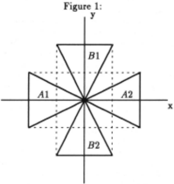
In order to apply bound propagation to any formula, it suffices to work bottom up in the formula tree com­ puting bounds which may be inferred from each terminal conjunctions of linear constraints, then grouping there­ sults for the disjunctions by selecting the less tightening bounds and so on until new bounds are computed for the root, i.e., for the whole problem. For example, if the formula (Al V A2) t... (Bl V 82) is considered where Ai and Bi are the triangles shown in figure 5.1, the first step of bound propagation yields the bounds represented by the box enclosed in the dashed lines. This example demonstrates that bound propagation can last forever:

its solution is (0, 0) and at each step the bounds are only reduced by a factor of 2.

In order to draw the best of such a method, it is im­ portant to propagate any new bound inferred at one level of the formula tree in its subtrees (i .e., to propa­ gate bounds under hypotheses in the part of the formula which holds under the same hypotheses). This may be done with the algorithm described below. The recur­ sive function propagate_bounds takes as arguments a set of initial Bounds for the variables, and a Formula. It returns either a set of bounds implied by Formula, or the information Unsolvable if the formula is discovered incompatible with the initial Bounds.

propagate_bounds{Bounds, Formula)

{

} if Formula is a single linear constraint for each variable x in this constraint update its bound in Bounds as described above and return the result (which may be Unsolvable) if Formula is a conjunction Formula1 and Formula2 repeat OldJJounds := Bounds Bounds := propagate_bounds(Bounds, Formula1) Bounds := propagate_bounds(Bounds, Formula2) until Bounds= Unsolvable or Old_Bounds =Bounds (or after n iterations) return Bounds if Formula is a disjunction Formula1 V Formula2 Bounds1 = propagate_bounds(Bounds, Formula!) Bounds2 = propagate_bounds(Bounds, Formula!) if (Bounds1 =Unsolvable) return Bounds2 if (Bounds2 =Unsolvable) return Bounds1 else return Bounds1 U Bounds2 (union of each intervals)

The propagation is started by calling this function with Bounds containing no restriction and Formula be­ ing the whole formula to be tested for satisfiability.

The practical implementation of this algorithm is in fact more incremental. At each disjunctive node of the tree, the Bounds1 and Bounds2 sets are cached. Then, whenever propagation of Bounds is requested for this node, only the new information contained in Bounds compared to Bounds1 (or Bounds2) is propa­ gated through Formula1 (respectively Formula2). Note that, at the end of the algorithm, Bounds1 (respectively Bounds2) may be regarded as the bounds which hold un­ der the hypothesis that the first {respectively second) al­ ternative ofthe disjunction have been chosen {and there­ fore that the whole path leading to this disjunction has been selected).

Despite its incompleteness, bound propagation up­ dated at each level of the search tree often reduces the combinatorial explosion in an important manner by dis­ covering soon that some alternatives may be suppressed.

5.2 Linear relaxation

Solving a simple conjunction of linear constraints is an easy matter thanks to algorithms such as the Simplex. Even if a problem of the class studied here contains dis­ junctions, it is possible to derive from it a new prob­ lem containing only conjunctions and whose solution set includes every solution to the initial problem. This is called a linear relaxation. Testing the solvability of a relaxation already gives important information: if the relaxation is unsolvable, then so is the initial problem.

Obviously, a tight relaxation, i.e., one whose solution set is as small as possible, is of great interest. In ge­ ometrical terms, a set expressed using disjunctions of linear constraints is not convex, whereas one expressed using only conjunctions is convex. The idea is then to use the convex hull of a disjunction for its relaxation. The linear constraints defining this convex hull can be computed symbolically, by using a variable elimination algorithm [Lassez and Lassez, 1991]. This is however to be avoided, because the number of constraints defining the convex hull may grow exponentially with respect to the number of constraints appearing in the disjunction.

Nevertheless, there exists an interesting construction adapted from Balas [Balas, 1985] which allows the con­ vex hull of a disjunction of linear constraint sets to be represented compactly by only adding new variables. It is presented here for a disjunction with two elements, but the extension to more elements is straightforward.

Let D be the set defined by {y I A1·Y ~ b1 VA2·Y ~ b2} (here A; are matrices and b; are column vectors) . Let x be an element of conv(D), the convex hull of D. Then there exist reals Yl and Y2, and positive rea:ls 61 and 62 such that x = 61Y1 + 62y2, 61 + 62 = 1 with A1Y1 ~ b1 and A2Y2 ~ b2 . Let x1 = 61Y1 and x2 = 62Y2· This yields the relaxation rel(D):

X X1 + X2 1 61 + 62 A1x1 < b161 A2X2 < b262

In the definition of rel(D), the positivity constraints on the 6; can actually be removed. This is one differ­ ence between Balas' result and the following theorem. Moreover, we have demonstrated it even for unbounded polyedron.

Proof 1 · ( ~) By the above construction.

• (¢:)Let c.z $ d be a constraint implied by conv(D). Then by Fourier's theorem there exist vectors A1 and A2 such that AiAi = c and Aibi $ d fori E {1, 2}. This, together with AiZi $ bi6i, gives c.Zi $ d6i, for i E {1, 2} . By summing these two constraints, we get c.(z1 + z2) $ d(61 + 62), As z = z1 + z2 and 61 + 62 = 1, this means that any point z of rei( D) verifies c.z $ d.

Now, any problem in normal form can be relaxed into a conjunction of constraints, using Balas' relaxation to remove each disjunction. Please note that, because of the conjunctions connecting different disjunctions with each other, it is not the convex hull of the solution of the global problem which is obtained, but instead a less tight constraint set.

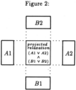
The example in figure 5.2 illustrates how from the in­ consistent formula (A1 V A2) 1\ (B1 V B2), the space of possible solutions is well reduced by the relaxation with­ out succeeding in discovering the inconsistency. Note that on this example bound propagation alone succeeds in proving inconsistency. However if the drawing is ro­ tated by 45°, bound propagation does not find anything, while Balas' relaxation will be as precise as without ro­ tation.

This linear relaxation is only one possible among many. It is however the only known one which is so tight without needing any complex computation. Relax­ ations for a disjunction of constraints which are currently used in Mixed Integer Programming (see for example [Williams, 1988]) introduce less new variables in the for­ mulation. However, they do not succeed in approaching the convex hull of the disjunctions. Balas' relaxation used here certainly adds many new variables, but be­ cause the average complexity of the Simplex is only pro­ portional to the logarithm of the number of variables, this is not a real problem. Moreover, as the added con­ straints are only equalities, they can be easily erased by substitution. Therefore, Balas' relaxation is both com­ putationally convenient and very precise.

5.3 Coupling bound propagation and relaxation

Balas' relaxation is perfect (i.e., represents the convex hull of the solutions) only when applied to one disjunc­ tion of constraint sets. However, it is in theory possible to build a convergent series of relaxations by:

• computing explicitly the projection on the initial z variables of the first Balas' relaxation (that suppose each variable Zi and 6i are removed by an ale;orithm such as the one in [Lassez and Lassez, 1991J).
• adding the result to each leaf of the formula tree
• and iterating, i.e., recompute a Balas' relaxation ...

Balas has demonstrated in [Balas, 1985] that such a series converges (in possibly infinite time) toward the convex hull of the solutions of the initial formula. This is completely impractical since just computing the pro­ jection may give an exponentially big result, which is to be duplicated and re-projected. Even so, this theoretical result is useful in showing the interest of "re-injecting" in the leaf of the tree the information about the global solution space. The only manageable information for this purpose is the bounds on the variables. Now, let us consider the bounds computed by the propagation for one leaf of the formula tree. By definition, these bounds can be added as explicit constraints to the correspond­ ing formula leaf without removing any potential solu­ tion. Then, if Balas' relaxation is consequently updated, it may become much tighter.

Finally, relaxation can be used to perform a "local enumeration". This means verifying that each 6i may be fixed to 1. If some 6i cannot be set to 1 then they are necessarily zero and the corresponding alternative should be suppressed. After such suppressions it is worth to restart the looking ahead phase at its beginning, i.e., bounds propagation.

6 Learning

By learning, we mean inferring general Boolean con­ straints over hypotheses, in order to reduce a priori unex­ plored paths of the search tree. Such constraints can be detected using two different methods: incompatibilities from bounds, and failure analysis. In both cases, these constraints are of the form -.(/\i6i)· During the con­ straint solving process, many of them can be inferred. They are stored in a symbolic Boolean constraint solver, or better in an ATMS [de Kleer, 1986]. Such an algo­ rithm is able to detect early that hypotheses are fixed (in the case of an ATMS, one-element nogoods), and man­ ages efficiently the constraints in store. Therefore, after many such constraints have been inferred, the possibili­ ties for the hypotheses 6i can be reduced drastically. For example, if 61 and 62 are known to be incompatible, if one of them is fixed to 1, then the choice corresponding to the other one will automatically be avoided.

6.1 Learning from bounds

Each bound computed by the bound propagation algo­ rithm can be labeled by the set of hypotheses yielding to it. When bounds for the same variable are incompatible with two different sets of hypotheses, for example, z $ 3 for 61 A 62 A 63 and z ~ 4 for 64, the conjunction of all the hypotheses is false. If an extended ATMS similar to the one described in [Dague et a/., 1991] is used, the bounds z ~ 3 and y ~ 4 are recorded along with their justifica­ tion. A new nogood { 61 , ... , 64} is then created, and the ATMS propagates this information, possibly discovering new nogoods.

6.2 Failure analysis

Relaxing a problem yields a set S of linear constraints over continuous variables and 6 variables. If it is un­ solvable, it is interesting to know why. This can easily be analyzed as being due to a subset of constraints in S which are incompatible together. This subset will be called a conflict. As each constraint is related to one hy­ pothesis 6;, a conflict may be easily translated in terms of hypotheses.

Let us first explain how a conflict in terms of con­ straints may be built. The solvability of the set S { A.z ~ b}, where A is a matrix, can be tested by com­ puting min zo on Ax + Is - l.z0 = b, where I is the identity matrix, s = (s1 , ... sn) is a vector of slack vari­ ables, z 0 is a positive variable, and 1 is a column vector whose coordinates are all equal to 1. S is solvable if and only if min zo = 0.

When S is unsolvable, the Simplex reaches a positive minimum value for zo with some variables in the ba­ sis (i.e., being not necessaraly stuck to 0). Constraints whose slack variables are not in this basis are the limits on which the minimization stumbled. They form a min­ imal conflict of S. As the reader can see, the detection of this conflict is done a posteriori, without any modifi­ cation of the core constraint satisfaction algorithm, i.e., at no cost. For a detailed presentation of this result see [De Backer and Beringer, 1991].

Once a cause of inconsistency has been found in terms of constraints, it can be translated in terms of the cor­ responding hypotheses. It can be added as a nogood in the ATMS, so that it can be used to further reduce the possibilities on the hypotheses. Please note that the minimality of a conflict in terms of constraints does not guarantee at all that the corresponding conflict in terms of hypotheses is minimal. However, it is usually not far from being minimal.

7 Comparison with other approaches

Many AI systems just use some kind of bound propa­ gation to draw information from any kind of arithmetic constraints. Depending on the application, the incom­ pleteness of such a method is more or less disturbing. For example, in a diagnosis application such as [Dague et a/., 1991], it may forbid to detect some failure cause. In any case, the hereabove tools may be fruitfully added to these systems when more completeness is necessary.

7.1 Mixed Integer Linear Programming

There exist many commercial packages able to solve Mixed Integer Linear Programming (MILP) problems, i.e., problems described by a simple conjunction of lin­ ear constraints in which some variables are forced to take integer values. The MILP formalism is powerful. In par­ ticular, the satisfiability of Boolean formulas over linear constraints may be transformed into a MILP problem.

Good MILP packages solve such problems by an im­ plicit enumeration method controlled by a Simplex and bound propagation. So even without any learning, they normally perform not too badly. However, when applied to problem naturally expressed in the disjunctive form studied here, they have an important limitation: they are not able to deal directly with the disjunctive for­ mulation. The user is then forced to reformulate com­ pletely the problem in MILP. This means that the user is in charge of generating the relaxation used by the al­ gorithm.

Now, though the relaxation proposed here is the most precise. one without being computationally·expensive, it cannot be used as such with MILP packages. Indeed, even after adding the constraints that the 6; variables are equal to either 0 or 1, this relaxation still has solu­ tions which do not correspond to solution of the initial formula. To obtain this essential property, many extra artificial constraints have to be added to enforce z; to be zero when 6; is zero. This is done by constraining each variable z; with two artificial bounds z; ~ M 6; and x; ~ -M6; where M is a large enough positive number. The resulting formulation has so many constraints that the Simplex may perform poorly on it. This is perhaps the reason why, despite its qualities, Balas relaxation has been hardly ever used.

Moreover, whatever MILP reformulation is chosen by the user, it hides the initial structure of the problem in such a way that bound propagation applied to this reformulation makes much less inferences than when it is applied directly to the initial formulation as proposed here.

Finally, no MILP package seems to use a learning tech­ nique similar to the one proposed here.

As a result, on difficult problems naturally expressed as Boolean formulas over linear constraints, our algo­ rithm should perform better than any MILP package running on any MILP reformulation.

7.2 Constraint Logic Programming

Languages as CLP('R.) [Heintze et a/., 1991] which extend the Prolog language with linear constraints may be used to express the satisfiability problem considered here, and even to solve it. However, used as such, the resolution algorithm handles very poorly the disjunctions: they are not considered in any way before branching on them.

But note that, when used to solve combinatorial prob­ lems, CLP languages are more programming languages than ready-to-use solving algorithms. As a matter of fact, the authors are currently testing and implementing the methods presented here using CLAIRE, a prototypal constraint extension of IBM Prolog.

8 Conclusion

Solving Boolean formulas containing linear constraints is a difficult combinatorial problem. As for any combina­ torial problem, there does not exist an "ideal" algorithm which would be better than the others on every prob­ lem. Success in combinatorial problem solving lies in the adequacy of the solving strategy to the restricted problem set to be solved. In particular, the user must have a way to specify heuristics able to guide the search. Indeed, success of Constraint Lo~ic Programming over finite domains [Hentenryck, 1989J may be explained by the ability to combine easily efficient algorithm thanks to a high level programming language.

The present work intended to provide basic procedures useful to design efficient algorithms while taking ada­ vantage of the problem specificities. The different pro­ cedures proposed here are not only separately efficient , but are also perfectly complementary. Thus, learning by failure analysis often gets an information which is not easily found by a priori analysis; Balas' relaxation is locally perfect but does not integrate long distance in­ fluences ; and, on the contrary, bound propagation is a rough approximation which takes into account the links in the overall problem.

The very first experiments with the prototype written in CLAIRE have shown good results. Further work will include the benchmarking of the method on problems of good size.