
Why AC-3 is Almost Always Better than AC4 for Establishing Arc Consistency in CSPs
Proceedings of the Thirteenth International Joint Conference on Artificial Intelligence. Constraint Satisfaction Problems. Pages 239-246.
© 1993 International Joint Conferences on Artificial Intelligence
Abstract
On the basis of its optimal asymptotic time complexity, AC-4 is often considered the best algorithm for establishing arc consistency in constraint satisfaction problems (CSPs). In the present work, AC3 was found to be much more efficient th~m AC-4, for CSPs with a variety of features. (Variable pairs were in lexical order, ~md in AC-3 they were added to the end of the list of pairs.) This is supported by arguments for the superiority of AC-3 over most of the nmge of constraint satisfiabilities ~md for the unlikelihood of conditions leading to worst-case perfonmmce. The efficiency of AC-4 is affected by the order of variable testing in Phase 1 ('setting up' phase); perform~mce in this phase can thus be enhanced, and this establishes initial conditions for Phase 2 that improve its performance. But, since AC-3 is improved by the smne orderings, it still outperforms AC-4 in most cases.
- [Dechter and Pearl, 1988] Dechter, R. and Pearl, J ., Network-based heuristics for constraint-satisfaction problems, Artif. lnte/1.34 (1988) 1-38.
- [Deville and Van Hentenryck, 1991] Deville, Y. and Van Hentenryck, P., An efficient arc consistency algorithm for a class of CSP problems, in: Proceedings /JCAI-91, Sydney (1991) 325-330. IJCAI
- Mackworth, 1977].
- A. Mackworth, Consistency in networks of relations, Artif.lntell. 8 (1977) 99-118. [Mackworth and Freuder, 1985].
- A. Mackworth and E. Freuder, The complexity of some polynomial network consistency algorithms for constraint satisfaction problems, Artif. lntell. 25 (1985) 65-74. Mohr and Henderson, 1986]
- Mohr, R. and T. C. Henderson, Arc and path consistency revisited, Artif. lntell. 28 (1986) 225-233.
- [Nadel, 1989] Nadel, B., Constraint satisfaction algorithms, Computational Intelligence 5 (1989) 188-224.
- [Perlin, 1991] Perlin, M., Arc consistency for factorable relations, in: Proc. IEEE Int. Conf. on Tools for AI, San Jose, CA (1991) 340-345.
- [Ullman, 1966] Ullman, J. R. Associating parts of patterns, Inform. Contr. 9 (1966) 583-601.
- [Van Hentenryck, 1989] Van Hentenryck, P., Constraint Satisfaction in Logic Programming, Cambridge, MA: MIT Press, 1989.
- [Wallace and Freuder, 1992] Wallace, R. J. and E. Freuder, Ordering heuristics for arc consistency algorithms, Proc . Ninth Canad. Conf on AI, Vancouver (1992) 163-169.
- [Waltz, 1975] Waltz, D. L., Understanding line drawings of scenes with shadows, in: The Psychology of Computer Vision, P. H. Winston, Ed. New York, NY: McGraw-Hill Book Company, 1975.
- [Williams and Hogg, 1992] Williams, C. P. and T. Hogg, Using deep structure to locate hard problems, in: Proceedings AAAJ-92 San Jose, CA (1992) 472-477.
References were extracted automatically from the PDF and may contain errors.
Full text extracted automatically from the PDF; figures, tables and equations may differ. The PDF is the version of record.
1 Introduction
Local consistency techniques c~m be used with search to improve the efficiency of algorithms that solve constraint satisfaction problems (CSPs). They have also proven useful in standalone implement:ttions, because they can yield solution sets or highly reduced problems [DeVille ~md Van Hentenryck, 1991]. The most common techniques establish arc consistency, i.e. , pairwise consistency for all variables in the problem or for a selected subset. This paper is concerned with algorithms that establish arc consistency for the entire problem.
AC-3 was introduced by Mackworth [1977] as a generalization ~md simplification of the earlier "filtering" algorithm of Ullman [1966] and Waltz [1975], now known as AC-2. Mackworth ~md Freuder [1985] showed that this algorithm has a worst case complexity bound that is significantly better than that of the simple strategy of scanning all pairs until no inconsistencies are found. Subsequently, Mohr and Henderson [1986] introduced AC-4 ~md showed that it has an even better worst case complexity, that is optimal in the general case.
This historical development has led to the impression that at each st:tge ~m algorithm was derived that was generally superior to previous algorithms in terms of efficiency [e.g., Perlin, 1991]. But since the main results are in terms of worst case asymptotic behavior, it is not clear that AC-4, the best algorithm in this sense, is actually better for a given problem or even better on average. It is possible that, for classes of problems, either AC-3 or AC-4 is superior. This is suggested by Van Hentenryck's [1989] remark that AC-4 is better for some problems, AC-3 for others.
*This material is based on work supported by the National Science Foundation under Grant No. IRI-9207633.
A related problem concerns the order in which variable domains are checked for consistency. It has been found that certain ordering heuristics can yield marked improvement in the performance of AC-3 [Wallace and Freuder, 1992]. For some problems, this might tip the scales in favor of this algorithm. On the other hand, it has been claimed (in personal communications) that AC-4 is "order-independent". If this were true, and if AC-4 was better than AC-3 for a given problem, it would not be necessary in this case to consider such ordering at all. Here it is shown that both AC3 and AC-4 provide opportunities for ordering to be effective, so these heuristics are important regardless of the algorithm chosen.
Section 2 describes the algorithms AC-3 and AC-4. Section 3 discusses average case performance under certain probabilistic assumptions. Section 4 gives results of tests of these algorithms on problems that differ with respect to key problem parmneters, including random problems and reduced queens problems. Large problems with parameter values that yield very difficult problems were also tested. Section 5 considers problems that result in worst case performance by AC-3 from a theoretical and empirical st:mdpoint. Section 6 discusses effects of ordering the Phase 1 list of variable pairs in AC-4, and presents empirical results for the problems of Section 4. Section 7 discusses problem classes in which the worst case complexity of arc consistency is less than 0(ed2). Section 8 presents conclusions.
2 Description of the Algorithms
A binary constraint satisfaction problem involves a set of n variables, vi, each with a domain of values, di, that it c~m assume. In addition, the problem is subject to some number of binary constraints, C ii· each a subset of the Cartesian product of two domains, di X di. A binary constraint specifies which pairs of values can be simultaneously assumed by the pair of variables. A CSP is associated with a constraint graph, where nodes represent variables and arcs or edges represent constraints.
AC-3 involves a series of tests between pairs of constrained variables, vi and vi. Specifically, values in di are checked against the constraint between vi and vi to see if they are consistent with at least one value in di; unsupported values are deleted. The AC-3 algorithm is shown in Figure l. All ordered pairs of constrained variables are ftrst put in Listofpairs. Each pair, (vi, vj), is removed and di is tested against dj- When values are deleted, it may be necessary to add pairs back to Listofpairs to detennine if these deletions lead to further deletions.
Initialize Listofpairs to {(vi, vj) I there is a constraint between vi and vj}. While Listofpairs is not empty Select and remove (vi , vj) from Listofpairs. Test vi against vi If any values are removed from di, add to Listofpairs any pairs (vk , vi), k~j. such that there is a constraint between vk and vi and (vk, vi) is not already present in Listofpairs. Figure 1. The AC-3 algorithm.AC-4 also begins with a sequence of tests between all pairs of constrained variables (Figure 2: Phase 1). But in this case the purpose of the tests is to determine mnount of support, i.e., how m<my values in the domain of vj support value a in the domain of vi and which values these are.
This infonnation is kept in special data structures for use in Phase 2 of the algorithm. If in the course of Phase 1, a value is found to have no support, this is recorded (in array Mark) and the value removed from the domain, as in AC-3.
After one pass through the set of variable pairs, AC-4 constructs a list of unsupported values (Listofbadvalues) in the form of variable-value pairs. Then, for each element on the list, (vk, c), the list of values supported by that value (collected in Phase 1) is exmnined. For each of the latter values, e.g., value d in the domain of Vf , the associated counter is decremented (here, counter [(vk , vf) d]). If a counter is decremented to zero <md the value was previously supported, it is put on the list of unsupported values. (Note. The present AC-4 [Figure 2] is identical to Mohr and Henderson [1986] except that in Phase 2 array Mark is checked before a counter is decremented rather tlkw after.)
3 Average Performance of AC-3 and AC-4
The following facts have been established regarding the time complexity of these algorithms. The worst case complexity of AC-3 is bounded above by O(ed3), where e is the number of constraints (edges) and d the maximum domain size [Mackworth and Freuder, 1985] . The time complexity of AC-4 is always O(ed2) [Mohr and Henderson, 1986]. Since the lower bound on the complexity of arc consistency is O(ed2), AC-4 is always optimal in terms of time complexity.
Another factor suggests that AC-3 would sometimes be more efficient than AC-4. In AC-3, each value in di is tested in terms of a yes/no query: is it supported by any value in dj or not? In AC-4 on the other hand, value testing involves questions of magnitude: how many values in dj support a value in d/? The latter query can only be answered by testing all values in dj rather than a sufftcient subset.
Initialize Listofpairs to {(vi, vj) I there is a constraint between vi and vj). For each (vi, vj) in Listofpairs For each value a in vi Set Total to 0. For each value b in Vj If a is supported by b in the constraint between vi and Vj Increment Total. by bin vi If Total= 0 Set Mark[ vi, a] to 1. Remove a from di. else Set counter for [(vi, vj) a) to Total .Add (vi, a) to list of values supported PHASE 2. Adjust counters to reflect deleted values, pruning other unsupported values. Initialize Listofbadvalues to those (vk, c) for which Mark[vk, c] = 1. While Listofbadvalues is not empty Select and remove (vk, c) from Listofbadvalues. For each (vz, d) in list of values supported by c If Mark[vz, d] = 0 Decrement counter for [(vk, vl) d] . If this counter is 0 Add (vl, d) to Listofbadvalues. Set Mark[ v 1 , d] to 1. Remove d from vl. Figure 2. The AC-4 algorithm .
The number of consistency checks between pairs of values (constraint checks) needed to determine if a value is supported can be estimated for random problems in which the probability that a value pair (a, b) is included in constraint C ij is p, and probabilities for different pairs are independent. Then the probability, p(k), that support for value a will be found after k constraint checks is,
If there are no supporting values, then ldjl tests will be made; the associated probability of this event is,
From these formulas the expected value of k, E(k), is
To give some concrete exrunples, suppose ldjl = 5. In this case AC-4 performs 5 constraint checks for each value tested against this domain. If p = .15, the expected number of constraint checks performed by AC-3 for each value is 3.7; if p = 0.3, the expected number is 2.8, if p = .45, the expected number is 2.1, and if p = .6, the expected number is 1.6. If ldil also has 5 values, the expected numbers of constraint checks for probabilities just given are 19, 14, 11 and 8, respectively, io contrast to 25 constraint checks for AC-4. Thus, across a wide range of inclusion probabilities, AC-3 performs less than half the number of constraint checks that AC-4 requires. In these cases, if AC-3 performs twice as many variable-pair tests as AC-4 does in Phase 1 it will still be more efficient. (Note also that on successive tests of the srune pair, the number of values checked will be smaller.) For random problems, especially when variable pair tests are ordered by a good heuristic, the number of variable pairs that must be retested is usually much less than this ([Wallace and Freuder, 1992], and see below).
4 Experimental Results
Evidence on the frequency with which AC-3 outperforms AC-4 <md the average difference in performance was obtained from empirical studies. Three kinds of CSP were exrunined:
- (i) random problems in which values for number of constraints (added to a spanning tree based on randomly selected constraints), domain size and satisfiability were chosen from the range of possible values, and then elements were chosen (at random) from the set of possible elements to equal the parruneter value. In the problems used here, n = 12, so 55 constraints could be added to a spannning tree. Thus, the number of added constraints could range between 0 and 55. Similarly, the maximum domain size= 12, and the value for a domain size was chosen between I and 12 inclusive. And for two domains with, say, 12 values, a value for the satisfiability of a constraint between them was chosen between 1 and 143 inclusive. These are called random panuneter value problems.
- (ii) random problems in which each element in the set of possible (additional) constraints, or possible domain values, or possible constraint pairs, was chosen with a probability that was constant for that parruneter. For ex<unple, in one set of ten-variable problems the probability for inclusion of a constraint was 0.1, for inclusion of a domain value the probability was 0.5 (maximum domain size = 10) and for inclusion of a constraint pair the probability was 0.35. This yields problems with, on average, about 14 constraints, five values per domain and a relative satisfiability of 0.35 per constraint. (Null domains and constraints were not allowed.) These are called random probability of inclusion problems.
(iii) k-queens problems with one domain (row) restricted to one or a few elements. This yields queens-like problems that can be reduced by arc consistency methods. Unlike the nmdom problems, constraint graphs are always complete.
R<mdom parameter value problems are heterogeneous internally, but average values for domain size and satisfiability are near the middle of the range. They are subject to considerable reduction by arc consistency methods. Probability of inclusion problems are more homogeneous with respect to their parruneter values, with average values close to those predicted from original probabilities. The runount of reduction due to violations of arc consistency is usually less than for random parruneter value problems. Five-queens problems with a domain restricted to one value show considerable domain reduction; with tO-queens the reduction is much less.
Ten twelve-variable random parameter value problems were generated in each of two constraint-ranges: 11-24 and 25-38. Five problems in each range with no solutions were also collected; lack of solution was detected by arc consistency algorithms in all cases, by domain 'wipeout'. Tests of these problems are referred to as Experiment I in the discussion of results.
Ten-variable probability of inclusion problems were generated with the following probability values: 0.1, 0.225 and 0.35 for constraint inclusion, 0.5 and 0.75 for domain value inclusion (maximum d = 10), and 0.35 and 0.55 for constraint pair inclusion. These factors were fully crossed, to produce twelve sets of problems. Five problems with solutions were generated in each category. Tests of these problems are referred to as Experiment 2.
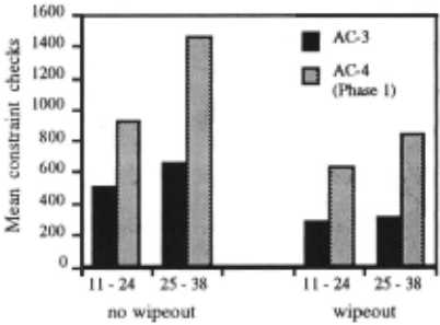
Figure 3. Performance of arc consistency algorithms on 12variable random parameter value problems. Number of constraint checks to produce consistency or wipeout.
Five- and ten-queens problems were tested, with the one domain restricted to one value or to either two (5-queens) or four (10-queens) values. The restricted domain was associated with either the first variable (first row), a middle variable (third or fifth row for 5- and 10-queens problems, respectively), or the last variable. All possible values were tested in the one-value cases, while five combinations of values were tested in each multi-valued case. These tests are referred to as Experiment 3.
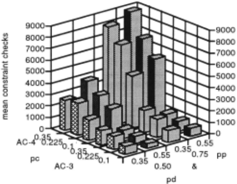
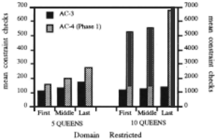
The relative performance of AC-3 and AC-4 in Experiments 1-3 was quite consistent (Figures 3-5). AC-3 outperfonned AC-4 on every problem tested, and the number of constraint checks was 2: 1 or better in most cases, even with comparisons limited to Phase 1 of AC-4. (Phase 2 does not use constraint checks.) AC-3 was, therefore, superior to AC-4 on problems differing in degree of difficulty, runount of domain reduction (ranging from no reduction to reduction to a single solution or to domain wipeout), key parruneter values, and systematic versus random patterns of dependency
(in the queens and nmdom problems, respectively).
Figures 3 and 4 show the expected effect on AC-4 of increasing the total number of values that must be checked, either by adding constraints or by increasing average domain size. At the same time, the effect of these changes on AC-3 is much smaller. For probability of inclusion problems, increasing constraint satisfiability (decreasing the tightness) also led to more constraint checks by AC-4. This was because there were fewer values deleted in the course of checking. But, consistent with the analysis in Section 3, decreasing the tightness led to fewer constraint checks by AC-3. This overcame the effect of fewer deletions, which is also a factor in AC-3's perfonnance.
Similar results were found with queens problems (Figure 5). Since the list was initially in lexical , order, these problems were progressively harder as the restricted domain was further back in the list. This was true for both algorithms, but the proportional increase was greater for AC-4. (The ratio of highest to lowest means was 1.55 and 1.17 for AC-3, for the 5- and 10-queens problems, respectively, and 1.75 and 1.29 for AC-4.) It seems that as a general rule AC-3 is less affected by problem features that produce more work for arc consistency algorithms.
In each experiment, differences in mean values were evaluated statistically by repeated measures analyses of variance, with algorithms as the repeated factor. (Separate analyses were done for problems with and without solutions in Experiment 1 and for 5- and 10-queens problems in Experiment 3.) For each test except that for the random parmneter problems without solutions, the algorithms factor was statistically significant at the 0.001 level. In the latter case, this factor was significant at the 0.01 level. In Experiment 2, the interaction of the algorithms factor with each of the three problem panuneters that were varied was statistically significant at the 0.001 level, reflecting the greater effect on AC-4. The factors based on probability of constraint inclusion <md domain element inclusion were themselves significant at the 0.001 level, while the factor based on constraint value-pair inclusion was not statistically significant. In addition, the interaction between the fonner two probability factors and the third-order interaction of these factors with the algorithms factor were significant at the 0.001 level. In Experiment 3, the factor based on location of domain restriction was significant at the 0.001 level in analyses based on the 5- or 10-queens problem, and the interaction between this factor and the algorithm factor was significant at the 0.01 level in both cases.
g
I·
For these problems, Phase 2 of AC-4 was done very quickly. In Experiment 1, the average number of badlist accesses was about 50, including 15 list additions, and there were about 300 Sjc (support list) accesses. In Experiment 2, there were few operations of any kind except for problems with small domains (p = 0.5) and small satisfiabilities (p = 0.35); even here, means for badlist accesses only varied from 15 to 40, with a mean of 2 to 16 additions, and means for Sjc accesses varied between 61 and 238. For problems with the largest domains and satisfiabilities, there was no domain reduction, so no work was required in Phase 2. For queens problems with singleton domains, there were 10 or 12 badlist accesses for 5-queens and 18 for 10-queens, while the average number of Sjc accesses was 22 and 382, respectively. For 2- and 4-valued domains, the number of operations of each type was reduced by a factor of five for 5queens problems, while no work was required for 10-queens problems since there was no domain reduction.
Two further experiments were run to detennine whether AC-3 would maintain its superiority with larger problems. In the first experiment, ten random parameter value problems were generated with 24, 48 or 72 variables. There was no restriction on number of constraints, and in all cases the maximum ldl was 12. After each problem was generated, a solution was added by selecting a value from each domain at random and, if necessary, replacing a value pair in a constraint with the pair that was consistent with this solution. Arc consistency reduced most of these problems to the added solution, with some exceptions among 24-variable problems. In the second experiment probability of inclusion methods were used to generate 99variable CSPs. The domain size was always four and the probability of value pair inclusion was 0.75, so they resembled four-color problems with respect to their parameter values. A range of densities was chosen that included a peak in the perfonnance curve, based on forward checking with dynamic ordering. This peak was near the "critical connectivity value" [Williams and Hogg, 1992]. It was, therefore, possible to compare AC-3 and AC-4 on inherently difficult as well as easy problems generated with the srune methods. In general, these problems did not admit much domain reduction. For this reason, similar problems with relative satisfiability equal to 0.5 were tested, in which peak difficulty was associated with a density of 0.005. These admitted more reduction, but the results for arc consistency were similar to the results for the first set of problems.
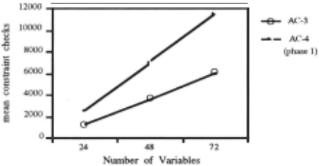
Results for the first experiment on larger problems are shown in Figure 6. Rather than decreasing as problems get larger, if anything, the degree of improvement with AC-3 increases. It should also be mentioned that, in testing AC-4, four 72-variable problems had to be run on a larger machine because of space requirements. In addition, as problem size increased, the amount of work required in Phase 2 became appreciable, ranging from a mean of 134 badlist accesses and 869 Sjc accesses for 24-variable problems to 406 badlist accesses and 3934 Sjc accesses for 72-variable problems. But performance was still dominated by Phase 1.
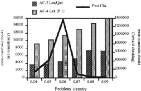
For 99-variable problems, AC-3 was markedly better than AC-4 at all problem densities, including those associated with hard problems. This suggests that the inherent difficulty of a problem bears no relation to worst case behavior of AC-3. And it confirms the conclusion of the previous experiment that AC-3 retains its superiority to AC-4 in the average case as problem size is 'scaled up'.
5 Worst Case Conditions for AC-3
Mackworth and Freuder [ I985] discuss the theoretical worst case condition for AC-3, in which each domain, di, is tested and reduced O(d) times, requiring the degreei-I implicated pairs of variables to be put back on the list on each occasion. They show that the total number of list additions in this case is d(2e - n), which, when multiplied by d2, gives an upper bound for worst case complexity. Their argument can be extended: if the total reduction is O(d) in each of O(n) domains, and if, for each of these domains, a reduction of O(I) occurs at the end of every set of O(degreei) tests against its constraining variables, then AC-3 will exhibit worst case behavior.
Problems that result in worst case perfonnance can be described in terms of sequential dependencies holding between values in different domains. For example, if value a in domain di of vi is supported by b in dj, and b depends in tum on c and din dk, then there is a sequential dependency from a to { c, d} via b. This can be shown by a restriction diagrrun [Wallace and Freuder, I992]:
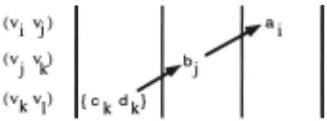
In a full diagrmn each column represents all values that can be eliminated at the beginning of testing or after all possible values have been eliminated in the previous column. There c~m . therefore, be up to 2e entries in a column.
Sequential dependencies can take many fonns. At one extreme (if any reduction is possible), there may be no indirect dependencies, and the restriction diagram has one column. The other extreme is a single dependency chain of length nd-I, whose restriction diagrrun has nd columns.
Obviously, if sequential dependencies allow enough domains to be reduced by O(d) in one stage (one column of the restriction diagram), then worst case behavior cannot occur. This can happen if one value supports O(d) values in another domain or if there is an effective branching factor in successive columns of the restriction diagram, e.g., value a in di is the sole support of values in two domains, each of which is the sole support of values in two domains, etc. Conversely, worst case conditions can only occur if the dependency relations are essentially I: I and the total length of the chains is O(nd).
If two dependency chains overlap with respect to the variables involved in a particular segment, there will be an ordering that allows deletions along both chains at the same time. If a sufficient number of chains are concurrent, then worst case conditions will be order- dependent; otherwise worst case conditions are order-independent.
For problems whose constraint graphs are trees, dependency chains cannot be longer than n-1, since a chain must end if a leaf-node is encountered. For, if the value deleted from the domain of that node were to support a value in the domain of a neighboring node, the latter value would have prevented deletion in the first place. This means that, for worst case tree-structured problems, the dependency chains must overlap; hence, worst case conditions for such problems are always order-dependent. There is, in fact, <Ul ordering for AC-3 that guarantees optimal perfonnance: for any node considered as the root of the tree, begin with the leaves and move toward the root, in each case testing parent against child and never testing a node farther from the root after testing one nearer. After the root has been checked against its children, proceed toward the leaves testing children against parents. With this ordering, if values ;:rre deleted when vj is tested against vi, other pairs (vk, vj)
will still be on the list. Hence, the complexity is O(ed2). (This is essentially the double directed arc consistency procedure described by Dechter ;:md Pe<rrl [1988].)
If the constraint graph has cycles, worst case conditions can be order-independent. But even in these cases the perfonnance of AC-3 may not be m;:rrkedly worse than AC-4 unless domains are very l<rrge. This is because the proportionality factor associated with O(ed3) perfonnance for AC-3 is always << 1, while for AC-4 the proportionality factor associated with O(ed2) perfonnance c;:m equal the maximum value of 2. Two independent factors improve AC-3's performance: (i) in worst case conditions domain sizes diminish with every set of tests, so the d2 term in the expression for worst case perfonnance, 2ed2 + d2(d(2e-n)) , must continually decrease, (ii) for a constraint between vi and vj, values in di will be tested against all values in dj only if there is no support or the sole support is the last value tested (using a ,standard test order). But this is incompatible with worst case conditions, since more than 0(1) values in dj could be deleted.
| a. Varying number of nodes (ldl = 10), | |||
| e AC-3 ccks | AC-3 (init list) Prop, Fact ccks 339 | .195 | AC-4 ccks 600 |
| 3 924 6 1884 | 669 | .203 | 1200 |
| 12 3804 | 1329 | .206 | 2400 |
| b. Varying domain size (n = e = 3). | |||
| ldl AC-3 ccks | AC-3 (init list) Prop. ccks | Fact J95 | AC-4 ccks |
| 10 924 20 5649 | 339 1279 | .182 | 600 2400 |
| 40 38,499 | 4959 | J75 | 9600 |
Note, Proportionality factor is AC-3 ccks for list additions divided by d2(d(2e-n))
Order-independent worst case CSPs were constructed with a single cycle of nodes and one long dependency chain
(beginning with ,the last variable pair in the lexical order) with n(d-1) elements. Table 1 gives results for different e and ldl. AC-3 is linear in e, and for these problems constraint checks were 50 % greater with AC-3 for each cycle 1ength. Appreciable differences in favor of AC-4 were only found when domains had 20 or 40 elements initially. For all problems the proportionality factor for AC-3 was 1/6 - 1/5. Interestingly, when ldl = 10, changing one constraint pair at random reduced the effort required by AC-3 to about that for AC-4, and with two such changes AC-3 was better. When ldl = 40, one or two random changes reduced the number of constraints made by AC-3 to about 20,000.
6 Effect of Ordering List of Variable Pairs
In the experiments discussed in Section 4, the list of v;:rriable pairs was ordered lexically, <Uld in AC-3 the list was thereafter treated as a queue. This appears to be the common procedure [Mackworth, 1977; Nadel, 1989]. However, it has been found that, for AC-3, ordering the list in tenns of basic p;:muneter values can have a marked effect on efficiency [Wallace and Freuder, 1992]. In this work it was shown that maintaining the list in order, by increasing size of the domain checked for support, is a very effective heuristic for reducing the number of constraint checks needed to achieve arc consistency. This heuristic is readily combined with an O(n) pigeonhole sort, leading to an overall efficiency that is superior to lexical/queue ordering. It has been asserted (in personal communications) that AC-4 is "order-independent". But, since Phase 1 of AC-4 is similar to the initial pass through the list of pairs in AC-3, it seemed likely that ordering heuristics found effective with the latter algorithm would also work with the fonner. In particular, order should matter because the same domain is often tested more than once; if values can be deleted sooner from this domain there will be a savings in the number of constraint checks. This is especially important in view of the fact that, in the experiments above, most of the work was done in Phase 1.
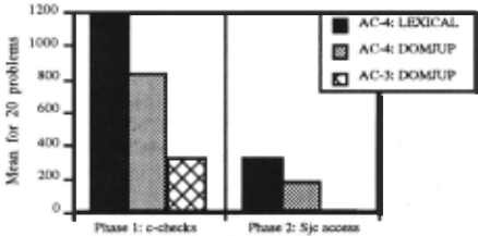
Phase 2, is less affected by ordering than Phase 1 because in the second phase there are no irrelevant tests. The only important exception is domain wipeout; early detection can obviously improve efficiency. Otherwise, the number of badlist and support list accesses is always the same for an initial set of badlist values, support lists and counters. (Unlike Mohr and Henderson [1986], the present implementation allows effects on counter decrements, because these are preceded by tests of array Mark; in limited tests such effects were very small.)
However, the number of operations can be significantly reduced in Phase 2 if the tallies are smaller at the beginning of this phase. This will occur if values are eliminated early in Phase 1, when they have not contributed very much to the tallies. Included in the first three experiments, therefore, were tests with an ordering heuristic based on increasing size of the supporting domain. This heuristic is called DOMJUP, retlecting the convention that the domain of vi is tested against the domain of vj.
In Experiments 1 and 3, us.e of the DOMJUP heuristic produced a marked decrease in the number of constraint checks required in Phase 1 (Figure 8. Similar results were obtained for random parameter value problems with no solutions and queens problems.) However, this did not make AC-4 as good as AC-3, since the latter's performance is also improved by the heuristic (For random parameter value and 10-queens problems, DOMJUP produced a greater proportional decrease in constraint checks for AC-3 than AC-4.) In both experiments, the Heuristics factor in the analysis of variance was significant at the 0.001 level. In the queens problems, the interaction of the Heuristics factor and the factor related to the domain restricted was also significant at the 0.001 level. This is because DOMJUP put domains most likely to be reduced at the front of the list in all cases.
In Experiment 2, where degree of domain reduction was much less, the improvement in constraint checks due to DOMJUP was slight, although it was still better on average even when only a few values could be deleted. But in this case the Heuristics factor was not statistically significant.
Figure 8 also shows that improved performance in Phase 1 of AC-4 led to improvement in Phase 2, measured by Sjc list accesses. As indicated above, this is because values that are deleted quickly are removed before they can be included in support lists for other values. Thus, even when order of testing bad values has little or no effect on the efficiency of Phase 2, this phase can be strongly affected by a 'ripple effect' from the ordering used in Phase 1.
7 Problems with Reduced Complexity
Recently it has been shown that there are certain classes of CSPs for which worst case complexity of arc consistency algorithms is O(ed). In some cases this is because domain support can be determined in one operation, for example, if the constraints are functional relations (actually bijections) [Deville <md Van Hentenryck, 1991]. In other cases this is because, (i) the values in a domain can be partitioned into equivalence classes, so relations can be factored into a set of relations based on these classes, (ii) there are bounds on the number of links between these classes [Perlin, 1991]. For bijectional constraints, the factors that make AC-4 less efficient in general are not present; in particular, the argument in Section 3 is not relevant. In this case, optimality considerations indicate that AC-4 should be used. On the other hand, ordering the list during Phase 1 can still improve efficiency. For factorable relations (condition (i) above), differences in efficiency should be reduced but not eliminated, so AC-3 may still be superior. If condition (ii) also holds, optimality considerations may again be the most important factor, although the relative superiority of the two algorithms remains an open question.
8 Conclusions
Although there is a small set of problems for which AC-3 is basically less efficient than AC-4, in practice the former algorithm is almost always more efficient for CSPs based on generalized relations. Worst case conditions aside, conditions which make arc consistency algorithms less efficient (greater number of constraints, larger domains) have a proportionally greater effect on AC-4 than on AC-3. When constraints have greater satisfiability, AC-4 is also less efficient while AC-3 is actually improved. If, in special cases, AC-4 is the preferred algorithm, then ordering the sequence of variable pair tests in Phase 1 can still improve the efficiency of this procedure, as it does for AC-3.
@inproceedings{ijcai1993p34,
  title     = {Why AC-3 is Almost Always Better than AC4 for Establishing Arc Consistency in CSPs},
  author    = {Wallace, Richard J.},
  booktitle = {Proceedings of the Thirteenth International Joint Conference on
               Artificial Intelligence, {IJCAI-93}},
  publisher = {International Joint Conferences on Artificial Intelligence},
  editor    = {Ruzena Bajcsy},
  pages     = {239--246},
  year      = {1993},
  note      = {Constraint Satisfaction Problems},
  url       = {https://ijcai.org/proceedings/1993/34},
}
TY - CPAPER TI - Why AC-3 is Almost Always Better than AC4 for Establishing Arc Consistency in CSPs AU - Wallace, Richard J. T2 - Proceedings of the Thirteenth International Joint Conference on Artificial Intelligence, IJCAI-93 PB - International Joint Conferences on Artificial Intelligence PY - 1993 SP - 239 EP - 246 UR - https://ijcai.org/proceedings/1993/34 ER -Copied
Machine-readable versions of this paper, for tools and AI agents:





