
Non-Order-Preserving Evaluation Functions: Recursive Graph-Search Methods for Job Sequencing Problems
Proceedings of the Thirteenth International Joint Conference on Artificial Intelligence. Planning. Pages 1423-1428.
© 1993 International Joint Conferences on Artificial Intelligence
Abstract
A* sometimes runs significantly faster than a tree-search branch-and-bound procedure if the search graph is represented as a graph and not as a tree. But graph search with A* is suitable only when the evaluation function is orderpreserving, i.e., in situations where a path in the explicit graph from the root to a node can be discarded when a better path to the node is found. 1bere exist interesting classes of problems, however, such as one-machine minimum-penalty job sequencing problems with sequencedependent setup times, for which the evaluation function is non-order-preserving. The search method cannot then discard any paths, and must store the entire explicit graph. GREC, a variant of an earlier recursive memory-constrained algorithm of the authors called MREC, has the desired properties and can be used in place of A•. Experimental results indicate that when the penalty is linear or quadratic, GREC is faster than tree search schemes and is able to solve problem instances of larger size.
- Bagchi and Mahanti 1983]
- A. Bagchi and A. Mahanti, Search Algorithms Under Different Kinds of Heuristics -A Comparative Study, JACM, vol. 30, no. 1, January 1983, pp, 1-21.
- Bell and Park 1990]
- C. E. Bell and K. Park, Solving Resource-Constrained Project Scheduling Problems by A• Search, Naval Research Logistics, vol. 37, 1990, pp. 61-84.
- Bianco et a/. 1988]
- L Bianco, S. Ricciardelli, G. Rinaldi and A. Sassano, Scheduling Tasks with Sequence 1428 Planning Dependent Processing Times, Naval Research Logistics, vol. 35, no. 2, 1988, pp. 177-184.
- S. French, Sequencing and Scheduling: An Introduction to the Mathematics of the Job-Shop, Ellis Horwood Ltd., 1982
- Korf 1985]
- Richard E. Korf, Depth-First Iterative Deepening : An Optimal Admissible Search, Artificial Intelligence, vol. 27, no. 1, 1985, pp. 97-109.
- Little et a/. 1963]
- J. D. C. Little, K. G. Murty, D. W. Sweeney and G. Karel, An Algorithm for the Traveling Salesman Problem, Operations Research, vol. 11, 1963, pp. 972-989.
- Mason and Anderson 1991]
- A. J. Mason and E. J. Anderson, Minimizing Flow Time on a Single Machine with Job Classes and Setup Times, Naval Research Logistics, vol. 38, no. 3, 1991, pp. 333-350.
- J. Pearl, Heuristics : Intelligent Search Strategies for Computer Problem Solving, Addison- Wesley, Reading, Mass., 1984.
- Ramaswamy and Sen 1992]
- Ramkumar Ramaswamy and Anup K. Sen, Single Machine Scheduling as a Graph Search Problem With Path-Dependent Arc Costs, Proc. ECA/-92, European Conference on Artificial Intelligence, Vienna, August 1992, pp. 11-15.
- Sen 1988
- Anup K. Sen, Heuristic Search Algorithms: A Theoretical-cum-Empirical Evaluation, Unpublished Ph.D. Thesis, Computer Science, University of Calcutta, 1988.
- Sen and Bagchi 1989]
- Anup K. Sen and A. Bagchi, F~t Recursive Formulations for Best-First Search That Allow Controlled Use of Memory, Proc. /JCA/-89, Detroit, August 1989, pp. 297-302.
- Sen and Bagchi 1993]
- Anup K. Sen and A. Bagchi, Job Sequencing with Quadratic Penalties: An A •-Based Graph Search Approach, Proc. CA/A-93, Conference on Artificial Intelligence for Applications, Orlando, March 1993, pp. 190-196.
- Sen et a/. 1991]
- Anup K. Sen, A. Bagchi and Bani K. Sinha, Admissible Search Methods for Minimum Penalty Sequencing of Jobs with Setup Times on One and Two Machines, Proc. /JCA/-91, Sydney, August 1991, pp. 178-183. IJCAI
- W. Townsend, The Single Machine Problem With Quadratic Penalty Function of Completion Times : A Branch and Bound Solution, Management Science, vol. 24, no. 5, 1978, pp. 530-534.
- Viswanathan and Bagchi 1988]
- K. V. Viswanathan and A Bagchi, An Exact Best-First Search Procedure for the Constrained Rectangular Guillotine Knapsack Problem, Proc. AAA/-88, American Association for Artificial Intelligence, St. Paul, August 1988, pp. 145-149.
- Viswanathan and Bagchi 1993]
- K. V. Viswanathan and A Bagchi, Best-First Search Methods for Constrained Two-Dimensional Cutting Stock Problems, Operations Research, May-June 1993, forthcoming.
References were extracted automatically from the PDF and may contain errors.
Full text extracted automatically from the PDF; figures, tables and equations may differ. The PDF is the version of record.
1 Introduction
In recent years, various attempts have been made to widen the range of problem areas to which Algorithm A · can be usefully applied. As part of this effort, A* has been employed to solve optimization problems in areas such as project scheduling (Bell and Park 1990] and rectangular stock cutting [Viswanathan and Bagchi 1988 1993]. In both of these cases the search graph is a tree, so there is little distinction between running A* and running a standard best first branch-and-bound procedure. In some application areas, however, such as in job sequencing and job scheduling (Sen et al. 1991, Ramaswamy and Sen 1992], far higher execution speeds have sometimes been achieved when the search graph has been represented as a graph instead of as a tree. Consider the optimal sequencing of jobs on one machine. It has been reported recently by Sen and Bagchi (1993] that Townsend's (1978] classic best-first branch-and-bound algorithm for minimal penalty sequencing of jobs when the penalty functions are quadratic runs 27 times faster for 16 jobs when implemented as an A · -based graph search scheme. The existence of such examples suggests that A* based graph search methods are likely to find greater use in future in the solution of sequencing, scheduling, stock cutting and related problems.
1 On leave from the Indian Institute of Management Calcutta.
But A· is not suitable for all types of one-machine job sequencing problems. One major difficulty that must be resolved when a job sequencing problem is formulated as an A· -search problem is that the evaluation function is sometimes found to be non-order-preserving (Pearl1984, pp. 100-102]. When the evaluation function is order preserving, a path from the root to a node can be discarded when a path of lower cost has been found. A · is based on this principle. But in the non-order-preserving case, no path can be discarded, because it is possible for a path that is currently unpromising to become promising at later stages of the search process. Suppose we allow jobs to have setup times. The setup time for a job is the time taken to get the machine ready for processing after the processing of the previous job has been completed and before the processing of the current job can begin. The setup time for a job J is sequence independent if it does not depend on which job is processed immediately prior to job J; otherwise, it is sequence dependent. When setup times are ignored or assumed to be sequence independent, A*-based graph search methods yield optimal solutions. When setup times are sequence dependent, however, the evaluation function becomes non-order preserving. Unfortunately, A* is not at all suited to the use of non-order-preserving evaluation functions, unless the search graph happens to be a tree. Graph search can sometimes be faster than tree search, and for a given memory, can solve problem instances of larger size. If these advantages are to be retained, the entire explicit graph needs to be stored, and an alternative algorithm must be found.
The MREC algorithm of Sen and Bagchi ( 1989] appears to answer the need. MREC is a constrained-memory graph search algorithm that can be viewed as a generalization of the tree-search scheme IDA* [Korf 1985]. Unlike A*, MREC
is recursive, and it does not use an OPEN list. All it needs is sufficient memory for its implicit stack:. But it can be fed at runtime a parameter M which tells it how much memory is available for use. In this memory, MREC stores as much as possible of the explicit graph. When M is large, MREC stores the entire explicit graph, and when M is small, MREC becomes identical with IDA ·. IDA · always makes a large number of node expansions. It runs fast on the 15-puzzle because with the Manhattan heuristic the time to expand a node is small. If node expansion time is significant, MREC is to be preferred over IDA*.
In this paper we explain how MREC can be employed to solve search problems with non-order-preserving evaluation functions. We proceed in three steps:
- First, we demonstrate the existence of important and interesting real life applications which are inconvenient to solve using graph search methods based on A* because the evaluation functions are non-order preserving. Tree search would solve the problems, but owing to duplication of nodes would run slowly and expand some nodes many times.
- ii) Secondly, we show that MREC(M = oo) can solve such problems. It would seem, therefore, that MREC(M = oo) has certain unexpected advantages over A ·. Since we are only interested in MREC when M is large, we give a new name to MREC(M = oo). We call it GREC. Note that GREC never expands a node more than once.
- iii) Thirdly, we propose new methods of solution for the linear penalty and quadratic penalty versions of the one machine minimum-penalty job-sequencing problem with sequence-dependent setup times. The quadratic penalty version of the problem has an inherent practical interest, but it is generally considered very difficult to solve, and this is perhaps the first time that a reasonably efficient method of solution is being proposed for it.
In section 2 we review the GREC algorithm, and in section 3 we introduce the one-machine minimum-penalty job-sequencing problem. Section 4 presents our solutions for the linear and quadratic penalty cases. We provide experi mental results in support of our claim that GREC runs faster than tree search methods and, for a given memory, solves problems of larger size.
2 Algorithm GREC
GREC is identical to MREC with the memory parameter M set to infinity. It outputs optimal solutions when heuristic estimates are admissible, never expanding a node more than once. Some of its important features are noted below.
- GREC is based on the recursive procedure EXPLORE, which, at each iteration, explores the explicit graph below the root node s. Initially the explicit graph contains only the root node. EXPLORE moves down a path in the explicit graph, making recursive calls to itself, until it encounters a tip node, i.e., a node which has no successors in the explicit graph. It expands the
program GREC; var terminate; begin (* initially the explicit graph contains the root nodes *) terminate := false; initialize s; (* b(s) = 0 *) repeat EXPLORE(s) until terminate; output b(s) as solution cait; output outpath as solution path; end. procedure EXPLORE(n:node); begin if n is a goal node then begin terminate := true; return; end; ifn is a tip node then EXPAND(n); UPDATE(n); end; procedure EXPAND(n:node); begin for each successor ni of n do end; ifni is not present in the explicit graph then begin initialize ni; (* b(Dj) = h(ni) *) add ni and the edge (n,ni) to the explicit graph; end else add the edge (n,Dj) to the explicit graph; procedure UPDA TE(n:node ); var cutoff : integer; begin cutoff := oo (* a very large value *); for each successor ni of n do begin if b(n) :2: b(ni) + c(n,ni) then begin b(ni) := b(n) - c(n,Dj); EXPLORE(ni); if terminate then begin add ni to outpath; return; end; end; if b(Dj) + c(n,ni) < cutoff then cutoff := b(ni) + c(n,ni); end; b(n) :=cutoff; end.tip node and adds the new nodes and edges to the explicit graph. As in IDA ·, a cutoff value is used for monitoring the downward movement. GREC terminates when it encounters a goal node.
- ii) Each node n in the explicit graph has a b-value b(n) which stores the current estimate of the cost of a path of least cost from n to a goal node. When n is a tip node, b(n) is set equal to the heuristic estimate h(n). The downward movement along a path is determined by the b-values of the nodes on the path. When GREC on reaching a node n finds a successor ni of n such that b(n) :o2: b(ni) + c(n,ni), it explores ni. If b(n) > b(ni) + c(n,ni), then b(ni) gets reset to a larger value, and this allows a deeper exploration below n. If b(n) < b(ni) + c(n,ni) for every successor ni, then none of the successors get explored. In this case, b(n) gets reset to the minimum of the b(ni) values. If n is explored at a subsequent instant, n will have a successor ni for which b(n) :o2: b(ni) + c(n,ni), and ni will be explored. The explicit graph thus grows in size, and more and more nodes and edges get added to it.
- iii) EXPLORE itself uses two procedures, EXPAND and UPDATE. EXPAND expands a tip node and adds newly generated nodes and edges to the explicit graph. UPDATE explores the graph below a node and updates the b-values of nodes. The algorithm stores the output solution path in outpath. The explicit search graph and its associated parameters are assumed to be accessible to all the procedures.
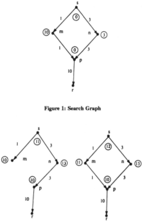
Example 1: For the search graph in Figure 1, we want to find the minimum cost path from the start node s to a goal node. The sequence of node expansions made by GREC is s n p m. A·, on the other hand, expands nodes in the sequence s n p m p, expanding the node p twice. Let each instant correspond to a fresh call to EXPLOREO with argument s; at the ith instant, EXPLORE(s) is called for the ith time. The explicit graphs at instant 3 and at termination of GREC are shown in Figure 2. In the figures, heuristic estimates and b-values of nodes are encircled. At instant 1, s gets expanded and b(s) gets updated to 6, which is the minimum of the two values c(s,m)+b(m) and c(s,n)+b(n). At instant 2, n gets explored. Since b(n) is 3 and c(n,p)+b(p) is also 3, p gets expanded, and the b-values of p, n and s are revised to 10, 13 and 11 respectively. At instant 3, m gets expanded and b(s) is revised to 12. At instant 4, GREC terminates with s m p r as the minimal cost path. D
Empirical results on a variety of problems indicate that GREC is very fast when evaluation functions are order preserving,. On the 8-puzzle problem with the Manhattan heuristic, it is as fast as IDA ·. On the travelling salesman problem using the evaluation function of Little et.al. [1963], and on tree search problems, it is as fast as A [Sen and Bagchi 1989). In problems where a node is expanded more than once and node expansion time is appreciable, it tends to be much faster than A· [Sen 1988). The power of GREC comes from the use of the b-value, which estimates the cost of the best path from the node to a goal; the b-value helps to determine whether further exploration below the node is worth pursuing, and is an extremely useful feature.
Comparing the properties of GREC, A* and IDA*, we find that:
- The sequences in which nodes are expanded by GREC and by A· are not the same.
- Unlike A·, GREC never expands a node more than once.
- When the heuristic estimate function is admissible, GREC always finds a minimal cost solution path. A · may not find an optimal path for non-order-preserving evaluation functions. Even for order-preserving evaluation functions, the optimal solution paths found by the two algorithms can differ. However, GREC and IDA · always output the same solution path.
- The worst-case running time of GREC, like that of A· and IDA·, can be exponential in the number of nodes in the search graph.
3 One-Machine Job-Sequencing Problems
A typical one-machine job sequencing problem has the following form. Jobs Ji with processing times ai, 1 :s; i :s; N, are submitted to a one-machine job-shop at time t = 0. The jobs are to be processed on the given machine one at a time. Let the processing of job Ji be completed at time~· Penalty jUnctions Gi(.), 1 :s; i :s; N, are supplied, such that the penalty associated with completing job Ji at time ti is Gi(ti)· An example of a penalty function is Gi(ti) = piti 2 , where the p/s are given constants, the penalty associated with a job being proportional to the square of the completion time of the job. The jobs must be sequenced on the machine in such a way that the total penalty
is minimized. The penalty functions are non-decreasing, and in general non-linear. Problems of this type have obvious relevance to industry, but are known to be hard to solve. In a more general setting, jobs have setup times. The setup time for a job is the time taken to get the machine ready for processing after the processing of the previous job has been completed and before the processing of the current job can begin. If Ji is the first job in the sequence, then its setup time is So,i· The setup time for job Ji when it immediately follows job Ji in the processing sequence is si,j· After the last job in the sequence is completed, the machine need not be brought back to any specific state. Setup times are said to be sequence independent (or separable or additive) if si,j can be expressed as a sum of two terms, one of which depends only on job Ji and the other only on job Ji; otherwise, the setup times are sequence dependent [French 1982, Bianco et al. 1988]. Branch-and-bound approaches frequently make the simplifying assumption that setup times are sequence independent (Mason and Anderson 1991 ]. Solution methods that work in the absence of setup times can frequently be extended to the situation when setup times are sequence independent. But if we make the more realistic assumption that setup times are sequence dependent, entirely new solution methods are typically required.
In the absence of setup times, A* solves many of the one-machine job sequencing problems efficiently. Let there be N jobs to be sequenced. Nodes in the search graph correspond to unordered subsets of jobs; the root node is the empty set. When a node corresponding to a subset of k jobs gets selected from OPEN and expanded, it generates N-k sons, each son being a subset of k + 1 jobs. An edge signifies that one more job has been processed, and the cost of the edge is the penalty associated with that job. A problem gets solved when a complete set of N jobs gets selected from OPEN. The method of computation of the heuristic estimate at non-goal nodes varies from problem to problem. In the sequence-independent quadratic penalty case, for instance, a very fast and memory-efficient implementation results if Townsend's (1978] method of computing the evaluation function is adopted [Sen and Bagchi 1993].
When setup times are sequence dependent, a different kind of search graph is needed. Nodes can no longer correspond just to subsets of jobs, because the last job that has been processed must be remembered. Thus a node now corresponds to an ordered pair, where the first component~ the job subset, and the second component is that job in the subset that has been processed last. As before, the cost of an edge is the penalty associated with the cor'responding job. A node n in the search graph has the form (S, J), where S ~ a subset of jobs and Ji is the last job processed from among the jobs inS. Let P 1 and P 2 be two paths from the root node s to n. The jobs processed along either of the two paths all belong to S. Let ti be the time at which Ji completes processing when the jobs in S are processed in the sequence determined by path P 1 , and let t'i be the time at which Ji completes processing when the jobs are processed in the sequence determined by path P 2 · When setup times are ignored or are assumed to be sequence independent, ~ always equals t'i· But when setup times are sequena: dependent, ti may not equal t'i· because the setup times of jobs along the two paths are not identical. It can happen that the cost associated with P 1 is less than the cost associated with P 2 , but ti > t' i. Since the penalty corresponding to a job depends on its time of completion, the arc costs of the arcs emanating from node n as well as the heuristic estimate at node n depend in general on the path by which n is reached from the root, i.e., the arc costs and the heuristic are path· dependent [Bagchi and Mahanti 1983]. It is also possible for a complete job sequence of N jobs that is an extension of the job subsequence determined by P 2 to have a lower total cost than a job sequence of N jobs that is an extension of P 1 · But a normal implementation of A · would discard path P 2 at node n because its cost is higher than that of P 1 , and job sequences that are extensions of the sequence determined by P2 would not subsequently get considered by the algorithm. In the linear penalty case, it is possible to skirt this difficulty by making a minor modification in A" [Ramaswamy and Sen 1992]; but the method does not seem to work in the quadratic penalty case.
| Job | Setup Times | Proc. Times | |||
|---|---|---|---|---|---|
| 1 | 2 | 3 | 4 | ||
| 1 | - | 1 | 1 | 00 | 1 |
| 2 | 1 | - | 3 | 00 | 4 |
| 3 | 00 | 00 | - | 10 | 3 |
| 4 | 00 | 00 | 00 | - | 10 |
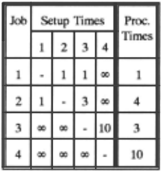
Example 2: Consider the following linear penalty problem with 4 jobs. Let the penalty coefficients be unity for all the jobs; then the penalty for a job Ji equals ti, where ti is the finish time of the job, and the total penalty is the sum of the individual job penalties. Table 1 gives the setup times and the processing times. Setup time si,j is the entry in the ith row and jth column of the table. The initial setup times So,j are assumed zero. The cost of the arc (m,r) between node m = ({1,2,3}, 3) and the goal node r = ({1,2,3,4}, 4) depends on the path by which we reach m from the root. If we process J 1 before J2 then the cost of the path P 1 from the root tom is 19, and c(m,r) = 32. If we process J2 before J1 then the cost of the path P 2 from the root to m is 20, and c(m,r) = 30. If at m we favor P1 and discard P2, then we end up giving preference to the inferior of the two solution paths. The minimum penalty job sequence in this case happens to be (J2 J1 J3 J4). D
4 Non-Order-Preserving Evaluation Functions
4.1 Linear Penalties
When penalties are linear and setup times are sequence dependent, a modified version of A· finds minimum penalty sequences [Ramaswamy and Sen 1992]. The same problem can be solved by GREC in the following way. When a node n = (S, Ji) first enters the explicit graph as a result of the expansion of its parent node, the completion time ti of n's last job Ji is saved in a parameter T associated with n. At a subsequent instant, if the EXPWRE procedure happens to reach n again, the completion time of job Ji has a value t'i which is in general different from ti because there are many paths from the root node to n. T must then be reset to t'i·
| Algorithm | No. of jobs | Exec. time (sees) | Nodes Gen. | Nodes Exp. |
|---|---|---|---|---|
| A• (Tree) | 12 | 0.04 | 710 | 93 |
| 14 | 0.13 | 1952 | 217 | |
| 16 | 0.39 | 4988 | 481 | |
| 18 | 1.33 | 14039 | 1182 | |
| 20 | 4.55 | 36818 | 2818 | |
| GREC | 12 | 0.02 | 333 | 64 |
| 14 | 0.06 | 657 | 119 | |
| 16 | 0.17 | 1329 | 225 | |
| 18 | 0.43 | 2563 | 415 | |
| 20 | 1.21 | 5400 | 842 | |
| 22 | 6.31 | 10475 | 1634 | |
| 24 | 35.36 | 18965 | 2836 |
The value of b(n) depends on the path by which n is reached from the root, and thus T plays a role in the computation of b(n). When T changes in value from ti to t'i· b(n) changes in value by the amount (t'i-~) }: ck, where we sum over those jobs which remain to be processed at n.
Example 3: Consider the job sequencing problem of Example 2. Let us assume for simplicity that all nodes have zero heuristic estimates. GREC outputs the minimum penalty sequence (J2 J 1 J3 J4) with cost equal to 50 without expanding any node more than once. The algorithm operates as described in Example 1. Suppose a node n has been reached from the root at some instant along a path P1. If n is reached from the root at a subsequent instant along another path P2, arc costs and b-values at n are recomputed with the help of the stored value of T. D
In our implementation, heuristic estimates at tip nodes were computed as in [Ramaswamy and Sen 1992]. Let n = (S, Ji) be a tip node in the explicit graph. Let Q be the set of jobs yet to be processed at n. For a job Jk in Q, take the effective setup time sk to be min{sjk}, where the minimum is taken over all jobs Ji in Q U g}. Let us call the (sk+aJ values the effective job processing times. Order the jobs Jk in Q in non-decreasing order of (sk+aJ/pk , compute the finish times tk of the jobs, and let the heuristic estimate be }:pktk, where the summation is over all jobs in Q. This yields a very good heuristic, as our experimental results in Table 2 show.
In the experiments, the programs were written in C and run on a UNIX-based DEC 5900 system. Processing times of jobs were integers and were chosen randomly in the range 1 to 99 from a uniform distribution. Penalty coefficients and setup times were integers in the range 1 to 9 and were generated in the same way. The initial setup times s 0 ,j were assumed zero for simplicity. For a given number of jobs, the execution time, the total number of nodes generated, and the total number of nodes expanded were averaged over 100 runs. The A· tree implementation was run upto 20 jobs. GREC was able to solve larger problems, and was about 3.76 times faster for 20 jobs than the A· tree procedure. Every effort was made to ensure that the implementations were as efficient as possible. The OPEN set of A· was maintained as a priority queue. In GREC a hashing scheme was used for checking whether a newly generated successor was already present in the explicit graph.
4.2 Quadratic Penalties
The elegant and efficient A· graph implementation of the quadratic penalty case that is realized using Townsend's [1978] method for computing the evaluation function does not appear to permit a generalization to sequence dependent setup times. To resolve this difficulty, GREC must be used in place of A ·. The method of solution is similar to that in section 4.1; some additional computations are needed at each step because the penalty function is non-linear.
At a tip node n, the effective processing time (sk+aJ for a job Jk in Q is computed as before. A heuristic estimate is then found for n by a modification of Townsend's [1978] method. The computation procedure for the heuristic is described in [Sen and Bagchi 1993]. In the UPDATE procedure, the b-value at a node n along the path of downward movement can be expressed as
where T, A, B and C are parameters that depend on node n. A, B and C do not depend on T. We have
- B = 2 }: { Pkt' k I Jk is in Q' },
and C can be viewed as the b-value at node n, where job completion times in B and C take n as the origin. A, B, and C must be stored at each node and get reset in UPDATE.
| Algorithm | No. of jobs | Exec. Time (sees | Nodes Gen. | Nodes Exp. |
|---|---|---|---|---|
| A• (Tree) | 12 | 0.15 | 3479 | 462 |
| 14 | 0.69 | 12857 | 1441 | |
| 16 | 3.38 | 49923 | 4957 | |
| GREC | 12 | 0.08 | 856 | 214 |
| 14 | 0.33 | 2159 | 512 | |
| 16 | 1.32 | 5067 | 1169 | |
| 18 | 12.16 | 12932 | 2954 | |
| 20 | 82.95 | 31750 | 7042 |
Experimental results are shown in Table 3. The tree implementation of A· also used the Townsend heuristic. GREC could be run for a larger number of jobs, and was about 2.56 times faster than A· tree search for 16 jobs. For 18 jobs, the tree search scheme generated more than 450,000 nodes in some instances. Since the number of computations at each step in the quadratic case is greater than in the linear case, running times in Table 3 are higher than in Table 2.
@inproceedings{ijcai1993p197,
  title     = {Non-Order-Preserving Evaluation Functions: Recursive Graph-Search Methods for Job Sequencing Problems},
  author    = {Sen, Anup K. and Bagchi, Amitava},
  booktitle = {Proceedings of the Thirteenth International Joint Conference on
               Artificial Intelligence, {IJCAI-93}},
  publisher = {International Joint Conferences on Artificial Intelligence},
  editor    = {Ruzena Bajcsy},
  pages     = {1423--1428},
  year      = {1993},
  note      = {Planning},
  url       = {https://ijcai.org/proceedings/1993/197},
}
TY - CPAPER TI - Non-Order-Preserving Evaluation Functions: Recursive Graph-Search Methods for Job Sequencing Problems AU - Sen, Anup K. AU - Bagchi, Amitava T2 - Proceedings of the Thirteenth International Joint Conference on Artificial Intelligence, IJCAI-93 PB - International Joint Conferences on Artificial Intelligence PY - 1993 SP - 1423 EP - 1428 UR - https://ijcai.org/proceedings/1993/197 ER -Copied
Machine-readable versions of this paper, for tools and AI agents:





