Planning Using Multiple Execution Architectures

1 Introduction

The goal of a decision-making system is to select the best action in the current situation. In a decision-theoretic frame­ work, this is expressed as choosing the optimal action, rf· , given the probability distribution on the outcome states, s E :,·, and a utility function on outcome states, u( s ):

If an agent can continuously apply this equation (decision theory's maximum expected utility (MEU) principle) to select "best" actions, it can be considered to be generating optimal behavior with respect to its goals. However, in even moder­ ately complex domains, the MEU Principle cannot be imple­ mented directly because of limited resource constraints (e.g., time) and uncertainty about the utility of outcome states. This paper discusses two general-purpose techniques used by the RALPH-MEA 1 agent architecture that alleviate this AI scala­ bility problem: multiple execution architectures and metalevel control of planning.

An agent can be defined as a function f : p· ___. D where p· is the set of percept sequences from the environment and Dis the set of action decisions available to the agent. An exe­ cution architecture (EA) [Russell , 1989) is an implementation of the agent function that operates on a specific combination of knowledge types (e.g., goals, probabilities of states, out­ comes of actions, etc.). Different execution architectures will have different competences and costs in different situations - for example, reactive condition-action rules are good for shooting down missiles and playing standard chess openings, but decision-theoretic planning may be more useful for select­ ing missile targets and playing tactically sharp middle games. Employing multiple EAs with the appropriate control to arbi­ trate the final action choice. should allow greater competence to be exhibited than is possible for a single EA alone.

'This research was supported by NSF granL~ JRI-8903146, lNT9207213, and CDA-8722788, and the Lockheed AI Center.

1 Rational Agents with Limited Performance Hardware-Mulliple Execution Architectures

The second tool we use to implement the MEU princi­ ple is metalevel control of planning. Planning is the method of projecting the current state into the future to predict pos­ sible outcomes. If the domain is simple enough, there is no need for planning since the the MEU principle can be applied with exact probability and utility functions for the action outcomes. However, as the domain becomes more complex, we need to consider subsequent action sequences in order to calculate the utility of the outcomes of our im­ mediate actions. Metalevel control of planning determines when and how much planning should be done. By view­ ing planning as a computational action, it can be integrated into the same decision cycle as base-level actions (i.e., ac­ tions that directly affect the external world). On each cycle, a best action must be selected, and it may be a base-level or computational action. Theoretical and practical issues of decision-theoretic metareasoning have recently been an active research area (e.g., [Russell and Wefald, 1989; Doyle, 1990; Henrion et al., 1991]). Our approach calculates a "value of information" [Howard, 1965] of doing various planning ac­ tions, selecting the planning or base-level action that has the highest utility.

First, we will discuss the representation used for multiple execution architectures and planning (section 2). Then we will describe the decision cycle that uses those representa­ tions to output action recommendations (section 3). Section 4 describes results from an autonomous, underwater vehicle (AUV) domain, implemented at the Lockheed AI Center.

2 Representation

2.1 Knowledge Types

Each execution architecture (EA) is a different representation of the agent function, f : p· -+ D, that outputs decisions. The EA categorization is based on the use of six types of knowledge. The original specification [Russell, 1989] of the knowledge types used a situation calculus representation, but in this paper, we introduce an extended influence diagram representation. An influence diagram explicitly accounts for the uncertainty of the states and provides inference algorithms to update beliefs given new evidence. An influence diagram represents actions as decision nodes, outcome states (includ­ ing goals) as probabilistic state nodes, and preferences among outcome states using value nodes. Depending of the node types they connect, the arcs in the influence diagram repre­ sent probabilistic, informational, or value dependence.

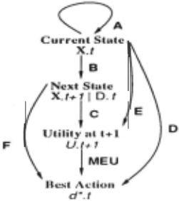
Our extended influence diagram (EID) representation dif­ fers from an influence diagram by defining the dependencies using the six types of knowledge. These dependencies are more specialized than the general probabilistic, informational, and value dependencies used in an influence diagram, and therefore, specialized inference procedures can be used rather than the standard influence diagram inference techniques.

To describe the current world state, we usc a set of n state variable nodes, X.t = {XJ.l , ... , .Y, .l}, a decision node D.t, and a utility node U.t. The suffix .l is used to indicate timet. For the next time, l + 1, the nodes arc represented as X.t+l = {X1 .t+1 , ... , .\, ./+IJ,adccisionnode /J./+1, and a utility node U.t+ 1. Assuming a Markov property on the states allows specification of the influences on X ./+ 1 using only X .t and D.t.

As is shown in figure 1, the six knowledge types of the EID representation, denoted by the lcners A, fl , C', D, E, F, connect the different knowledge components together. These six knowledge types arc given decision-theoretic definitions as follows:

A: p(X; .tjX.t)

Type A rules specify the likelihood or a state node given information about other sLate nodes for the same Lime. Rules of this type can be used for the interpretation of percepts. For example, the dependence of the variable FuelGauge.t given the percept BatteryFailure.t can be represented as a conditional probability function: p(Fue/Ga.uge.t I Balle7·yFa-ilu1·e .I).

8: p(X;.t+lJD.t, X .t )

Type B rules describe the effects or actions by specifying the influence of an action on the resulting state. In con­ trast to a type A rule, an action f) .t and conditions X .I at time t influence the node .\"; .1. + 1 at time I+ 1. The example p(DataAcc1'ued.1JD.O, DataAccrued.O) states that the node Da.taAccrued.l of time 1 is directly affected by DataAcc1'ued.O and D.O of time 0.

C: v(U.t+1JX.I+1) E [u.l.,uT)

Type C rules are utility functions on the state. In the EID, this is represented using a value function von the node U.t+ 1 which is bounded by the minimum and maximum possible utilities, u.l. and u T.

0: v(U.l+1j1J.t,X.t) E {u.l,uT}

Type D rules are akin to standard condition-action rules used in reactive or production rule systems. They state that if the specified conditions hold now, then the specified action is best. The utility U.t + 1 is conditioned on X.t and D.t of time t. Type D rules express absolute certainty by using the endpoints of the utility range as their only possible values.

E: v(U.t+1JD.t,X.t) E [u.l.,uTJ

Type E rules are "action-value" rules that specify the utility of condition-action pairs, for example Q-tables [Watkins, 1989]. In the EID representation, they represent the same qualitative influences as D rules but the utility value is generalized to the range [0, 1).

F: v(U.t+1JX.t+1) E {u.l.,uT}

The type F rule, which is similar to a classical goal [Newell, 1982], expresses the utilities of states in the future time period, t + 1. The utility is restricted to u.l. or u T values. A desirable goaliswhen v(U.t+1JX.t+1) = uT.

2.2 Execution Architectures

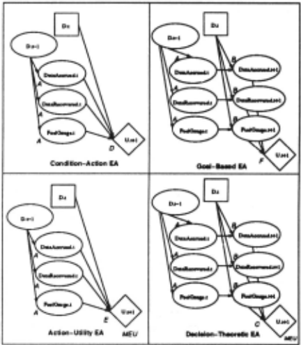
Exactly four execution architectures can be defined using the four different combinations of knowledge types to make an action decision (figure 2).

CA: Condition-Action EA: (path A D)

Knowledge of type D provides best action choices directly. In many production systems, uncertainty regarding the pre­ conditions of a rule is not considered. A precondition either is true or false, and the action of any rule whose precon­ ditions are matched is executed. This type of system can be implemented by the Condition-Action EA by allowing no uncertainty about the conditions (p(Xi.t!X .t) E 0, 1). The Condition-Action EA then would output the first action, d;, it considers such that v( U.t+ II f) .I = d;, Y .t) = uT (the max­ imum possible utility) and the rule's preconditions hold. The alternative Condition-Action EA implementation is to allow uncertainty about the preconditions. However in this case, the expected utilities of each action must be computed and compared to select the best action. Computational savings can still be achieved by taking advantage of the restriction of utility values to the minimum and maximum possible utilities: { u l., u T}. For example, if u l. = 0, many propagations of values in the EID are immediately pruned.

GB: Goal-Based EA: (path A 13 F)

Knowledge of types A, B, and F suggests actions that achieve the desired goal condition. Similar to the case with the Condition-Action EA, two possible implementations of the Goal-Based EA can be considered. If the probability values of conditions are restricted to 0 and I, the first action satis­ fying the goal utility function is selected. If uncertainty of conditions is allowed, the expected utilities of actions need to be computed, but computational savings results from the restriction of utility values to { u l. , liT} .

AU: Action-Utility EA: (path A E MEV)

Knowledge of type E for various actions is combined with the MEU principle to select the most valuable one. Inference in the Action-Utility EA uses the standard probabilistic and decision-theoretic reasoning techniques done in inlluence di­ agrams: the conditional probabilities of each state node arc revised by propagating the ellcct of evidence through the net­ work, the expected utility of each action is computed, and the action with the maximum expected utility is selected. The Q-tables from Q-Iearning [Watkins, 1989] are knowledge of type E.

DT: Decision-Theoretic EA: (path ABC MEV)

Knowledge of types A, B, and C is combined to find the best action using the MEU principle. As in the Action-Utility EA, standard decision-theoretic reasoning needs to be used in the Decision-Theoretic EA because of the lack of restrictions on the possible utility values.

In order to succeed in complex environments, an agent will need all four execution architecLUres, which will come into play at different times. If we consider chess, for example, it seems obvious that action-utility rules have restricted use­ fulness (perhaps just for describing the value of exchanges, knight forks etc.); condition-action rules constitute the "open­ ing book", some endgame knowledge and perhaps plausible move generators; goal-based reasoning occurs when identi­ fiable goals (such as checkmate, trapping a queen, queening a pawn etc.) become achievable with reasonable likelihood; and the remaining situations are covered by decision-theoretic planning using a utility function on states (material, center control etc.). It would be absurd to try to build a chess program based entirely on condition-action rules or action­ utility rules, because such a program would be unimaginably vast. Compact representations of good decision procedures require a variety of knowledge types. It would also take a long time to learn a complete set of condition-action rules for chess, whereas it takes only an hour or two for a human to learn type B rules describing how the pieces move. This provides another motivation for multiple execution architec­ tures: learning is more effective for the explicit knowledge types (A,B,C) but execution is more efficient for the compiled types (D,E,F); thus we learn for one architecture and compile, where reasonable, for another2.

2.3 Planning windows

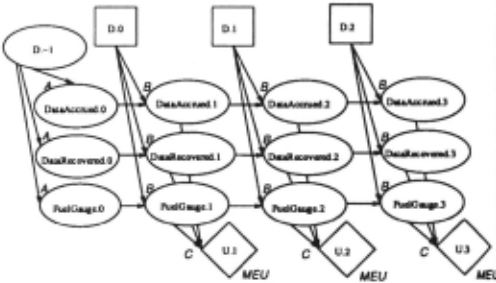
For an action sequence rather than a single action, many single-decision templates like the ones of Figure 2 can be chained together. Assuming the Markov property of the states, we can reproduce the same decision template repeatedly as the world stale is projected forward in time using only local connections. The planning window is the influence diagram that is currently being considered. For one-step planning, the length of the window is one time step. For k-step planning, the influence diagram is extended by chaining k decision tem­ plates together.

Figure 3 shows a 3-step planning window obtained by chaining together three decision templates of the Decision­ Theorelic EA in a simplified version of the autonomous un­ derwater vehicle (AUV) domain. The utility of the AUV's mission is defined in terms of whether it recovers survey data (nodes: DataAccrued and DataRecovered) and the amount of fuel used (node: FuelGauge). The decision node D.t has three possible actions to choose from: wait, wail for data to accrue at the sensor; return, return to the surface to be recovered; and pickup, go to the sensor to pick up the data. The decision node of the previous time, D.t -1, becomes evidence for the next decision, D.t.

The utility of the action sequence in general can be a func­ lion of all the nodes in the planning window, however, a common restriction is to make the action sequence utility a function of the utilities at each time slice (e.g., in figure 3, the utility of the (D.O, D.1, D.2) sequence would be a function of the utility nodes U.1, U.2, U.3). Another method is to eval­ uate the action sequence using only the utility of the final time slice (e.g., U.3).

2 ln [Ogasawara, 1993] we show general conditions under which learning action-utility values (e.g., Q-learning [Watkins, 1989]) works bcucr or worse than learning the utilities of states.

It should be noted that planning windows apply only to the Goal-Based EA and Decision-Theoretic EA. The Condition­ Action EA and the Action-Utility EA do not contain knowl­ edge describing the effects or actions (Type B knowledge), therefore, there is no way to chain together single deci­ sion templates. Also, "planning" in this decision-theoretic framework is somewhat different from the traditional no­ tion of planning for goal achievement. The aim of plan­ ning is no longer to achieve goals but to maximize ex­ pected utility. As has been often pointed out, the gener­ ality of maximizing expected utility rather than achieving goals is necessary to deal with multiple objectives and goal achievement uncertainty (e.g., [Feldman and Sproull, 1977; Wellman and Doyle, 1991)).

3 The Decision Cycle

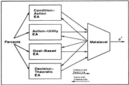
Given the execution architecture and planning window rep­ resentation, there is still the issue of how to usc the four execution architectures together H) make decisions. Our cur­ rent implementation works as follows. Corresponding to each of the four EAs, there is a separate influence diagram that is executed in parallel to determine an action recommendation for that EA. A separate Meta level influence diagram receives updates from the four EAs and makes the final decision on the action choice by checking the values of a "best action" node. At this stage of the research, this method has the ad­ vantage of modularizing the EAs to allow the design and performance of individual EAs to be isolate<1 3 · The Meta level is also separated from the implementation of the EAs and can be developed independently. Figure 4 shows the high-level system architecture view of RALPH-MEA.

The decision making algorithm follows a cycle in which the following computation occurs:

1. The model is update<! by advancing the planning window and entering new evidence.
2. Each EA computes its action choice.

3 Later versions will combine the separate Extended Influence Diagrams in order to share nodes.

1. Instantiate last executed action node, D.t, as evidence.
2. Add new time slice t + k + l.
3. Integrate out nodes of timet (X.t, D.t, U.t).
4. Set t = t + 1.
5. Enter new evidence for X.t nodes.
6. Propagate evidence through network.

Figure 5: The Updating the Model step.

1. The Metalevel ID determines when to stop the EA com­ putations and output the current best action.

The following sections examines each of these steps in turn 4 ·

3.1 Updating the model

As the agent makes decisions, the planning window is updated by modifying the influence diagram. After D.t is executed, its value is instantiated as evidence. For a k-step planning window, a new time slice is added by connecting nodes of time t + k to the new nodes of time t + k + 1. Nodes of time t, X.t , D.t, U.t, are then removed from the network by integrating their values into the rest of the network. In general this is done by converting the conditional probabilities p(X; .t+ liX.t) into marginal probabilities:

The time variable t is then incremented so that the next decision to execute is again D.t. Evidence for the new X.t nodes in each EA influence diagram is entered at this point. For example, if we detect a battery failure, the corresponding node Bat teryFailure. t is set to True. Finally, prop­ agation is done to transmit the effects of the new influence diagram and new evidence to all the nodes.

Similar techniques have become common recently in the uncertainty community. [Kjaerulff, 1992) discusses an im­ plementation of "model reduction" and "model expansion" that moves a belief network forward in time, allowing a con­ tinuously existing agent to maintain an updated world model indefinitely 5 . [Kanazawa and Dean, 1989), [Hanks, 1990], and [Nicholson, 1992] also discuss similar temporal projec­ tion methods.

3.2 EA Computation

As each EA computes using its separate influence diagram, it modifies its assessment of the utilities of the possible actions. These action utilities are periodically read by the Metalevel ID to update its assessment of the action utilities and to de­ termine when to stop computing and output the current best action. The EAs run in parallel and if the Metalevel decides to execute its current best action before some EA has finished its computation, the EA is interrupted to start the next decision cycle.

4 Because of space limitations, many important details have been omitted, but can be found in [Ogasawara, 1993].

5 This assumes that the dependency structure remains fixed (e.g., there is no addition or removal of arcs or nodes)

1. R = U.t + k
2. Compute VJ(,·cp/a.n(X)) for each subtree X of R.
3. Xmax = argmaxx(Vf(rcplan(X))
4. if (VI(replan(Xmax)) :S 0) then d· .t = next plan step; exit. else if (Xmax is a decision node) then change its action value; goto 1. else R = X max; goto 2.

Figure 6: The EA Computation step.

It is in this EA Computation step that we consider planning actions to change the choice of base-level actions. We assume the planning window is initialized with a nominal plan that specifies a defaull action for each D . i in the planning window. The expected utility if the next plan step were executed is the current utilityofthc u. t +k node since the nominal plan steps are "programmed" in by initializing the prior probabilities of the corresponding decision nodes to near I for the actions of the nominal plan. The utility of executing the next plan step is compared to the utility of executing a planning action. The value of planning may be positive, for example, if there is new evidence since the plan was constructed or if the plan can be easily improved.

As our possible planning actions, we consider replanning decisions affecting different portions of the utility model in the influence diagram. For example, in figure 3, the direct influences on the utility node U.3 arc the Dola.-\ccrued .3, DataRecovered.3, and fuc/Cr'au.yc.3 nodes. We seck LO work on repairing the anributc nodes that will yield the max­ imum net utility gain, that is, the nodes with the maximum value of replanning.

Each node is the root of a subtree of other nodes that influence it. Suppose we determine that replanning the Fue/Gauge .3 subtree in the influence diagram has the high­ est estimated value of replanning. Recursively, the value of replanning the subtrees of FuclC:auge .3 are computed, and continuing in this manner the influence diagram is examined until (I) a decision node is reached and modified to the action value that maximizes utilityar(2)all examined subtrees have a negative estimated value of replanning.

Let X be the root of the subtree we arc considering re­ planning. Assuming that we can separate the time-dependent utility, TC(X), from the "intrinsic" utility, Elh (X), the es­ timated value of information (\if) gained from replanning subtree X is

where replan( X) denotes the action of replanning subtree X and~ indicates an estimated quantity.

The estimated utility of replanning a portion of the influence diagram EU 1(X) is computed by taking the utility difference between the the subtree after replanning, X', and the current subtree, X. To compute the utility for.\"', we must know the probability that difl"crent S 's will occur as a result or replanning. For a decision node, because it is completely controllable, the probability is I that any particular value can be achieved and simply the action value that maximizes utility is selected. But for chance nodes, we estimate the probability and update it based on replanning experiences.

• 1 . Do propagation for the current values to compute EU(d· .t).
• Do propagation to compute EU(d· .t').
• EVC(6t) = EU(d· .t')- EU(d· .t)- TC(6t)
• If (EVC(6t) :S 0) then execute d· .t; exit. else goto 1.

Figure 7: The Metalevel Computation step.

As an example, suppose X is the subtree rooted at Fue/Gauge .3. The utility of the current probability distri­ bution of Ftte1Gauge .3 node can be computed directly. But to compute the utility of the same node Fuei(Jauge.3' after replanning decisions that might change its probability distri­ bution, we must estimate how likely it is that the replanning will alter actions in the plan to achieve a new distribution F-ue/Ga1tge .3'. In the example, if the initial probability dis­ tribution for Fue/Gauge.3 has ahighprobabilityforthe value empty, the utility of that subtree will be relatively low. Bul if we know that there is a high probability that replanning (perhaps by omitting actions to lower fuel consumption) will change the probability distribution to more heavily weight half- full, the utility of the Fue/Gauge .3' subtree will be higher. Thus EU J(X) would be positive.

If the estimated value of replanning, V !(replan( X)), is positive, the replanning action with the highest value is ex­ ecuted, and the EA computation step is repeated with lhe new plan by comparing executing the next plan step and ex­ ecuting a planning action. When the value of replanning is non-positive, the EA computation step finishes with the nexl plan step as its action choice.

3.3 Metalevel computation

The metalevel problem is to take the computed results (in this case, the action utilities) of the four EAs and to outputa final action choice. At any time with its current information, the Metalevel ID has a current best action d· .t. As the resulls from the EAs arrive asynchronously, the Metalevel must de­ cide whether to execute the current best action d· .tor to wail 61 for possible updates from the EAs. This is the basic met· alcvel computation algorithm described in [Horvitz, 19881. [Breese and Fehling, 1988] also discuss a metalevel control architecture that uses multiple reasoning methods, but in their case, a particular method is chosen and then only that method is executed rather than combining the results of the methods.

The Metalevel ID is first used to compute the expected utility of the optimal action, EU(d· .t), by using the current running time of the decision cycle to instantiate the Time node, propagating the current evidence from the EAs through the network, and determining the optimal action DM L = d· .t and its expected utility UML = EU(d·.t). This calculation requires a measure of the "quality" of the computed results of the EA as a function of the time spent computing, tc. that is, a "performance profile" for each EA as a function of tc. We define the performance profile to be the probability that the decision that a particular EA would take after tc is the same decision that would be taken by the metalevel.

Using the same method, the expected utility of the optimal action after waiting 6t, EU ( d· .t'), is also computed by setting the node Time to the sum of the running time of this decision cycle and an increment !!..t.

The expected value of waiting tlt is

If EVC(!!..t) ~ 0, then there is no benefit in waiting and the current best action, d* .t, is executed. However, if EVC(!!..t) > 0 then we should wait for more computation by the EAs and repeat the meta level computation step.

4 AUV Example

We have implemented examples (300-400 nodes) of mul­ tiple EAs and planning windows for the AUV domain and have been encouraged by the results. For the implementation, we use the HUGIN software [Andersen et al., 1989] which operates only on probabilistic belief networks [Pearl, 1988]. Therefore, the extended inllucnce diagram is converted to a corresponding belief network as in [Cooper, 1988J by convert­ ing decision and value nodes into probabi I is tic state nodes. On top of the HUGIN software, we have written C code to im­ plement the multiple execution architectures framework and metalevel control of planning.

Since each EA has a different "performance profile" (deci­ sion quality as a function of computation time), in the multiple EAs implementation an interesting interaction that occurs be­ tween EAs as computation time varies can be observed. In our implementation, the Condition-Action performance pro­ file quickly rises to a medium level of decision quality, while in contrast, the Decision-Theoretic performance profile has a higher decision quality but only after a longer period of computation. Therefore, as computation time increases, the results of the Condition-Action EA arc weighted less, and the results of the Decision-Theoretic EA arc more heavily weighted. For a given situation, the Metalevcl's best deci­ sion may change several times as the EA computation time increases. Complex decision-making behavior is thus gen­ erated by specifying simple probability and utility functions and exploiting the modularity of the EAs.

We have also implemented the value of replanning mech­ anism and have seen it successfully replan when various dy­ namic events occur and successfully not replan when there is no or little benefit to be gained. In one example, after the execution of the first step of the nominal plan, a battery failure occurs. This event causes the value of replanning the Fue/Ga·u.ge subtree to be positive, and after recursively computing values of replanning in the network, a decision is changed from waiting two cycles for data to accrue to waiting zero cycles, thereby reducing the usc of fuel for the mission.

5 Conclusion

Two techniques used by RALPH-MEA to facilitate decision­ theoretic reasoning were discussed. The Multiple execution architectures framework uses performance profiles to com­ bine the information from four different implementations of the agent function to output an action choice. Decision­ theoretic planning uses a projectiblc decision template to construct a planning window. Within a planning window, the value of replanning is calcu latcd to provide metal eve I control over planning and execution.

We are currently building a more complex model of the AUV domain to use for decision-making. As the model be­ comes more complex, the need for multiple EAs and decision­ theoretic planning become more important, so we expect to get more impressive results from metalevel control. We are also working on acquiring and learning more accurate assess­ ments of the requisite probabilities and utilities needed (e.g., the performance profiles).