
Characterizing and Automatically Finding Primary Effects in Planning
Proceedings of the Thirteenth International Joint Conference on Artificial Intelligence. Planning. Pages 1374-1378.
© 1993 International Joint Conferences on Artificial Intelligence
Abstract
The use of primary effects of operators in planning is an effective approach to reduce search costs. However, the characterization of "good" primary effects has remained at an informal level. In this paper we present a formal criterion for selecting useful primary effects, which guarantees planning efficiency, completeness, and optimality. We also describe an inductive learning algorithm based on this criterion that automatically selects primary effects of operators. Both the sample complexity and the time complexity of our learning algorithm are polynomial in the size of the domain.
- [Bacchus and Yang, 1991] Fahiem Bacchus and Qiang Yang. The downward refinement property. In Pro- ceedings of the International Joint Conference on Ar- tificial Intelligence, pages 286-291, 1991.
- [Chapman, 1987] Planning for conjunctive goals. Artifi- cial Intelligence, 32, pages 333-377, 1987.
- [Carbonell et a/., 1990] Jaime G. Carbonell, Craig A. Knoblock, and Steven Minton. PRODIGY: an in- tegrated architecture for planning and learning. In Architectures for Intelligence, ed.: Kurt VanLehn, Erlbaum, Hillside, NJ, 1990.
- [Fikes and Nilsson, 1971] Richard E. Fikes and Nils J. Nilsson. STRIPS: a new approach to the application of theorem proving to problem solving. Artificial In- telligence, 2, pages 189-208, 1971. IJCAI
- [Fink and Yang, 1992a] Eugene Fink and Qiang Yang. Formalizing plan justifications. In Proceedings of the Ninth Conference of the Canadian Society for Com- putational Studies of Intelligence, pages 9-14, 1992.
- [Fink and Yang, 1992b] Eugene Fink and Qiang Yang. Automatically abstracting effects of operators. In Proceedings of the First International Conference on AI Planning Systems, pages 243-251, 1992.
- [Fink and Yang, 1992c] Eugene Fink and Qiang Yang. Planning with primary effects. In preparation, 1992.
- [Knoblock, 1990] Craig A. Knoblock. Learning abstrac- tion hierarchies for problem solving. In Proceedings of the Eighth National Conference on Artificial In- telligence, pages 923-928, 1990.
- [Knoblock, 1991] Craig A. Knoblock. Automatically Generating Abstractions for Problem Solving. PhD thesis, School of Computer Science, Carnegie Mellon University, 1991. Tech. Report CMU-CS-91-120.
- [Wilkins, 1988] David Wilkins. Practical Planning: Ex- tending the Classical AI Planning Paradigm, Morgan Kaufmann, CA, 1988.
- [Yang and Tenenberg, 1990] Qiang Yang and Josh Tenenberg. ABTWEAK: abstracting a nonlin- ear, least commitment planner. In Proceedings of Eighth N a tiona/ Conference on A rf ificial Intelligence, pages 923-928, Boston, MA, 1990.
References were extracted automatically from the PDF and may contain errors.
Full text extracted automatically from the PDF; figures, tables and equations may differ. The PDF is the version of record.
1 Introduction
1.1 Planning with Primary Effects
Planning with primary effects is an effective approach to reduce search costs. The idea of this approach is to select primary effects among the effects of each operator and to use an operator only when we need to achieve one of its primary effects. A primary-effect restricted planner never inserts an operator in a plan in order to achieve any of the side effects of the operator. For example, the primary effect of lighting a fireplace is to heat the house. If we have lamps in the house, we could consider illumi nating the room as a side effect of lighting a fireplace. We would not use a fireplace just to illuminate the room.
The advantages of using primary effects in planning are well-known. If a planner considers only operators whose primary effects match a current goal, the branch ing factor of search can be reduced. This may result in an exponential reduction of running time. For this reason, primary effects are used by many implemented planning systems, such as SIPE [Wilkins, 1988], PRODIGY [Car bonell et a/., 1990], and ABTWEAK [Yang and Tenen berg, 1990]. Besides, primary effects play an important role in systems that automatically generate abstraction hierarchies. Recent work [Knoblock, 1991], [Fink and Yang, 1992b] has shown that the use of primary effects allows us to increase the number of levels in abstraction hierarchies, resulting in hierarchies that in many cases increase the efficiency of abstract planning.
*School of Computer Science, Carnegie Mellon University, Pittsburgh, PA 15213. Email: eugene@cs.cmu.edu. The au thor is supported in part by a scholarship and grants from the Nat ural Sciences and Engineering Research Council of Canada.
tDepartment of Computer Science, University of Wa terloo, Waterloo, Ont., Canada N2L 3Gl. Email: qyang@logos.waterloo.edu. The author is supported in part by grants from the Nat ural Sciences and Engineering Re search Council of Canada and ITRC.
Despite the importance of primary effects, the char acterization of a "good". selection of primary effects has remained at an informal level. Most systems rely on a human user to select primary effects. If the user has not chosen primary effects, then by default all effects are as sumed to be primary.
A lack of a formal guideline for selecting primary ef fects could cause two serious problems in planning. First, an improper selection of primary effects may result in the loss of completeness in planning. Incompleteness happens when a primary-effect restricted planner can not find a plan for a solvable planning problem. For example, if a fireplace is the only source of light, but lighting is not chosen as a primary effect of using fire place, a primary-effect restricted planner will not find a plan to illuminate the room. Second, primary-effect re stricted planning may produce non-optimal plans. Thie happens because primary effects place a bias in directing the search for a solution. If not set properly, the bias can favor a search path toward a more costly solution.
Recently we have developed an algorithm, MARGIE, for automatically selecting primary effects [Fink and Yang, 1992b]. Although in many cases this algorithm leads to a dramatic improvement in running time, our experiments revealed that the above two problems some times cause a planner to perform worse than without the use of primary effects.
1.2 Overview of the Results
The purpose of the paper is twofold. First, we pinpoint the exact reason for a primary-effect restricted planner to be incomplete and non-optimal. This result is presented in the form of a theorem, which states a necessary and sufficient condition for a primary-effect restricted plan ner to be admissible. The theorem formalizes the intu itions behind "good" choices of primary effects. Using the theorem, it is now possible to determine whether a given selection of primary effects enables a planner to be complete and admissible.
| I operator | preconditions | I effects | cost |
|---|---|---|---|
| go(x, y) | robot-in~)) door(x, y | robot-mJ~( 3 -.robot-in x) | 2 |
| carry-ball(x, y) | robot-in~ x) ball-in(x) door(x, y) | robot-in_(Y) -.robot-in( x) ball-in(y) -.ball-ii~(x) | 3 |
| throw(x, y) | robot-in~ x) ball-in(x) door(x, y) | ball-in_(Y) -.ball-in( x) | 2 |
| break(x, y) | robot-in( x) | robot-in_(y) -.robot-in( x) door(x, y) | 4 |
Second, for incomplete or inadmissible choices of pri mary effects we present an inductive learning algorithm to automatically find additional primary effects. The learned set of primary effects guarantees a planner's com pleteness and ensures its ability to find a near-optimal solution. To use the learning algorithm, an initial set of primary effects can be chosen by the user or by an ini tialization algorithm. The learner then analyzes either a collection of previous plans or new plans generated by the planner to augment the set of primary effects of op erators.
The utility of our inductive learning algorithm is demonstrated by its time complexity and sample com plexity. The former characterizes the running time of processing a set of sample plans, while the latter speci fies the number of sample plans required by the learner to reduce the probability of planning errors to a small user-defined number. We show that the time complexity of our algorithm is polynomial in the size of the domain, and the sample complexity is linear in the total number of effects in operator definitions.
2 A Motivating Example
2.1 Planning Domain
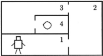
We describe a planning domain with a robot, which may move within four rooms (see the picture), and a ball in Room 4. The robot may go between two rooms con nected by a door, and it may carry the ball. Also, the robot may throw the ball through a door into another room. If two rooms are separated by a wall, the robot may break through the wall to create a new door.
To describe a current state of the domain, we have to specify the location of the robot and the ball, and pairs of rooms connected by doors. This may be done with three predicates, robot-in(x), ball-in(x), and door(x,y).
Literals describing a current state of the domain may be obtained from these predicates by substituting specific room numbers for .r and y. For example, the literal robot-in(!) means that the robot is in Room 1, ball-in(4) means that the ball is in Room 4, and door(l,2) means that Room 1 and Room 2 are connected by a doorway.
The operations performed by the robot, such as mov ing between rooms or throwing the ball, are called oper ators. Each operator a is described by a set of precon ditions Pre( a), a set of effects Etf(a), and a real-valued cost (see the table). The preconditions of a are the con ditions that must hold before the execution of the oper ator, and the effects are the results of the execution. If 1 is a member of Eil(a), then we say that a achieves l.
A plan is a sequence of operators that achieves some desired goaP. For example, assume that the initial state is as shown in the picture, and we wish to bring both the robot and the ball into Room 3. This goal may be achieved by the plan (break(1,4), carry-ba11(4,3)) . A plan is correct if (1) all goal literals are achieved, and (2) the preconditions of every operator a of the plan are satisfied before the application of a. We define the cost of a plan as the sum of the costs of its operators. The cost of our plan is 4 + 3 = 7. An optimal plan is one that achieves the goals with the minimal cost.
2.2 The Completeness Problem
If an operator has several effects, we may choose certain "important" effects among them and insert the operator into a plan only for the sake of these effects. Intuitively, an effect is not important if it may be achieved by some other, less expensive operator. The chosen important effects are called primary. Using primary effects in plan ning restricts the branching factor of search, which may improve efficiency.
For example, consider the following selection of primary effects:
go(.r,y) {robot-in(y)} carry-ball(.r, y) {robot-in(y) , ball-in(y)} throw(.r, y) {ball-in(y)} break(.r,y) {door(.r,y)}
Assume that the initial state is as shown on the picture and the robot must go into Room 3. The robot may achieve this goal by breaking through the wall between Rooms 1 and 3. However, since changing the location of the robot is not a primary effect of breaking through a wall, a planner will not consider this possibility. Instead, it will find the plan (go(1,2), go(2,3)).
The planner is not as fortunate when we consider an other goal: to remove the robot from Room 1. The for mal description of this goal is {-.robot-in(!)} . This may be achieved by the operator go(1,2) or, less efficiently, by break(l,3). However the planner will not find either of these plans, because -.robot-in is not a primary effect of any operator. Therefore, the planner will report that the goal cannot be achieved. This shows that planning with primary effects may not be complete, that is, it may fail to find a plan for an achievable goal.
1 In this paper we consider total-order plans. However, our results can be easily generalized to partial-order plans.
To preserve completeness, we have to add some additional primary effects to our selection:
go(x, y) {robot-in(y), --.robot-in(x)} carry-ball(x, y) {robot-in(y), ball-in(y)} throw(x,y) {ball-in(y), --.ball-in(x)} break(x,y) {door(x,y)}With this modification the planner is complete. However planning with these primary effects may still prevent us from finding an optimal plan. Suppose that we want the robot to go from Room 1 to Room 4. The goal may be achieved by the operator break(1,4), the cost of which is 4. However, entering Room 4 is not a primary ef fect of this operator, and a planner will not apply the operator. The best plan that the planner may find us ing primary effects is (go(1,2), go(2,3), go(3,4)), with the cost 6. This example demonstrates that planning with primary effects may not be admissible, that is, it may fail to find an optimal plan.
In the following sections, we formalize the notion of planning with primary effects and present a technique for ensuring the completeness and admissibility of planning.
3 Formalizing Primary Effects
3.1 Primary-Effect Restricted Planning
A planner is called primary-effect restricted if, when it inserts a new operator to achieve a goal or a precondition of another operator, it always uses an operator with a matching primary effect. To describe the completeness of a primary-effect restricted planner, we need to define a number of key concepts.
We first define the notion of justification. Informally, an effect I of some operator a in a plan II is justified if achieving I by a is required for the correctness of II.
Definition 1 An effect I of an operator a in a correct plan is justified if either
- I is a goal, and no operator after a achieves I, or
- I is a precondition of some operator a 11 such that one of the effects of a1 is justified and no operator between a and a 1 achieves I
Observe that the operators that do not have justified effects may be removed from the plan without violating the correctness of the plan [Fink and Yang, 1992a]. In this paper we assume that all operators of every plan have justified effects.
Definition 2 A correct plan II is primary-effect justi fied if every operator of II has a justified primary effect.
One may verify that if a planning problem has a primary-effect justified solution, then the primary-effect restricted versions of many planning systems, such as STRIPS [Fikes and Nilsson, 1971], TWEAK [Chapman, 1987], and PRODIGY [Carbonell et al., 1990], will find a solution to the problem.
Definition 3 Primary-effect restricted planning is com plete if, for any initial state So and goal state S 9 , the existence of some plan that achieves S 9 from So always implies the existence of a primary-effect justified plan that achieves S 9 from So .
Our next concern is the optimality of primary-effect justified plans. To describe the possible loss of efficiency when using primary effects, we introduce the notion of the greatest cost increase. A positive real number Cis called the greatest cost increase for a given selection of primary effects, if for any goal achieved by any plan II, there exists a primary-effect justified plan for achieving this goal, with the cost no greater than C · cost(II).
For example, consider the plan in the last example of Subsection 2.2. The optimal way for the robot to travel from Room 1 to Room 4 is to break through the wall, with the cost 4. However, the best primary-effect justified plan is to go through Rooms 2 and 3, which costs 6. Thus the cost increase for this problem is 6/4 = 1.5.
The greatest cost increase is the factor we will use for judging the degree of optimality for a given selection of primary effects. Its value is always greater than or equal to 1. The smaller its value, the better the selection of primary effects.
3.2 Necessary and Sufficient Condition of Completeness
To address the problem of selecting primary effects, we present a theorem that allows us to test whether a given choice of primary effects guarantees the completeness of planning and to estimate the greatest cost increase.
Let S be a state and a be an operator whose precon ditions are satisfied in S. A plan 111 with the initial state S is called a replacing plan for a in S if 111 is a primary-effect justified plan such that
- Il1 achieves all side effects of a, and
- 111 leaves unchanged all literals of S that are not changed by a
For example, consider the stateS = {robot-in(!), ball in(4)} and the operator break(l,4). The side effects of this operator are robot-in(4) and -.robot-in(!). A replac ing plan for break(l,4) is 111 = (go(1,2), go(2,3), go(3,4)), since Ill achieves both side effects of break operator and does not change any other literals of S.
The replacing cost increase is the ratio of the cost of an optimal replacing plan Il1 to the cost of a, coettn, . cos a In our example the cost of break is 4, and the cost of IT1 is 6, and thus the replacing cost increase is ~ = 1.5.
Theorem 1
[Completeness] Primary-effect restricted planning is complete if and only if for every state S and for every operator a whose preconditions are satisfied in S, there exists a replacing plan.
[Optimality] For a given complete selection of primary effects, the greatest cost increase equals
The second part of the theorem states that the greatest cost increase is equal to the maximum of replacing cost increases when the latter is greater than 1. Otherwise, it equals 1.
Sketch of the proof We prove the second part of the theorem, that the greatest cost increase is equal to the maximum of replacing cost increases. The proof of the first part is similar.
Let Cr be the maximal replacing cost increase. We have to show that (1) the cost increase for every plan ning problem is at most Cr, and (2) there is a planning problem for which the cost increase is exactly Cr.
{1) Consider an arbitrary planning problem with an initial state So and a goal S 9 , and an optimal plan II = ( a 1, .. , an) that achieves the goal. We have to show that there exists a primary-effect justified plan achieving the same goal, with the cost no larger than Cr · cost(TI). We may convert IT into a primary-effect justified plan by replacing some of its operators. We begin by consider ing the last operator, an . If it is not primary-effect justi fied, we replace it with the corresponding replacing plan. Since Cr is the largest replacing cost increase, the cost of the replacement is no larger than Cr·cost(an)· We repeat this process for the rest of the operators, an-1. an-2, and so on, until all operators without justified primary effects are replaced by primary-effect justified plans. It may be shown that when we replace some operator a;, all operators after it remain primary-effect justified. So, after we replace all n operators, we obtain a primary effect justified plan the cost of which is no greater than Cr · cost(a1) + .. + Cr ·cost( an)= Cr · cost(TI) . We con clude that the cost of an optimal primary-effect justified plan that achieves S 9 from So is at most Cr · cost(TI), and therefore . the cost increase is no greater than Cr.
(2) Consider an operator a and a state S such that the replacing cost increase of a in S is Cr , the largest of the replacing cost increases. Consider a planning prob lem with the initial state S and the goal to achieve all side effects of a and to preserve the values of all liter als not changed by a. The goal may be achieved by a single operator a, and thus the cost of an optimal plan is no greater than cost(a) . On the other hand, an opti mal primary-effect justified plan that solves the problem is a replacing plan for a in S, and therefore its cost is Cr ·cost( a). Thus, the cost increase is at least Cr . 0
The theorem can be applied to check whether a given choice of primary effects ensures the completeness and near-optimality of a primary-effect restricted planner, by examining each operator in the domain and finding a re placing plan for the operator's side effects. The theorem can also be used to design a learning algorithm that auto matically finds primary effects. We present our learning algorithm in the next section.
4 Automatically Finding Primary Effects
We would like to minimize the number of primary effects in order to limit the branching factor of search, but the selected set of primary effects must be large enough for ensuring the planner's completeness and optimality. Our algorithm is designed to ensure both of these criteria. The initial phase of the algorithm attempts to minimize the number of the primary effects. Then a learning com ponent augments the selected set to ensure completeness and optimality.
4.1 Initial Selection of Primary Effects
First, all user-defined primary effects are taken as a part of the initial selection. Then the algorithm ensures that every literal is a primary effect of at least one operator. Thus, the algorithm makes each literal I be a primary effect of some operator. Since we wish to minimize the cost increase of planning with primary effects, the algo rithm chooses the operator with the minimal cost among all operators achieving/. The corresponding procedure, InitiaLChoice, is presented in Table 1. Here the func tion User-Defined_Eff adds primary effects chosen by the user. The function CheapesLOperator(l) finds the minimal-cost operator a among the operators achieving I. If no operator achieves l, CheapesLOperator returns "not-found".
Example Suppose that InitiaLChoice is applied to our robot domain, and the user has chosen robot-in(x) and -.robot-in(y) as primary effects of carry-ball(x, y). The procedure finds the cheapest operators for the remaining literals, ball-in, -.ball-in, and door. The cheapest opera tor that achieves the literals ball-in and -.ball-in is throw, and the cheapest operator for door is break. Thus, Ini tiaLChoice selects the following primary effects:
| go(x,y) | none |
| break(x,y) | {door(x,y)} |
| throw(x, y) | {ball-in(y) , -.ball-in(x)} |
| carry-ball(x, y) | {robot-in(y) , -.robot-in(x)} |
4.2 Learning Additional Primary Effects
The learning algorithm augments the set of primary ef fects chosen by the procedure InitiaLChoice. It asks the user to provide the greatest cost increase C. The value of C is the cost increase that the user is willing to accept. Then the algorithm randomly generates example plans and tests whether every example plan IT may be replaced with a primary-effect justified plan nl that achieves the same goal, with the cost no greater than C · cost(TI). If such a plan ll1 cannot be found, the algorithm selects additional primary effects for the operators.
Our method may be viewed as an inductive learning algorithm. At any moment of learning, the current se lection of primary effects is the hypothesis of our learn ing method. Example plans are produced by a random example generator. An example plan IT is a positive ex ample if the planner finds a replacing primary-effect jus tified plan with the cost at most C ·cost(TI) that achieves the same goal as IT. If a replacing plan cannot be found, the example is negative. Our inductive learner ignores positive examples. For each negative example, it im proves the hypothesis by selecting new primary effects.
Processing One Example Plan The learning algo rithm selects additional primary effects by analyzing cor rect plans. Given an initial state S0 , a goal S 9 , and a plan n that achieves the goal, the algorithm converts IT into a primary-effect justified plan that achieves S 9 , with the cost no greater than C · cost(TI). (Recall that C is the greatest cost increase set by the user.) If the selected primary effects do not allow such a conversion, the learner selects additional primary effects.
To obtain a primary-effect justified plan, the algorithm considers each operator a of IT without justified primary effects and calls the procedure Prim-Eff-Planner to re place a by primary-effect justified plan ITt, such that the cost of ITt is at most C ·cost( a). If the replacement found by Prim_Eff-Pianner does not achieve all justified effects of a, then the learner chooses some justified ef fect 1 of a that is not achieved by the replacing plan and makes 1 a primary effect of a. After all operators are processed and new primary effects are selected as neces sary, the learner obtains a primary-effect justified plan that achieves S 9 · These operations are performed by the procedure Process-Plan shown in Table 1.
Example Let us apply the learning algorithm to our robot domain, with the initial selection of primary effects from the previous example. We choose C = 1.5 and con sider the single-operator plan (go(1,2)) with the initial state as shown on the picture and the goal { robot-in(2)}. Since the operator go does not have primary effects, this plan is not primary-effect justified. So the learner calls the planner Prim_Eff-Planner (see line 3b of the algo rithm) to find a primary-effect replacement for go. The planner fails to find a primary-effect justified plan to achieve the goal, and the learner chooses robot-in(y) as a primary effect of go(z, y). Thus, the selection of primary effects becomes as follows:
go( z, y) {robot-in( z)} break(z,y) {door(z,y)} throw( z, y) {ball-in(y), ...,ball-in( z)} carry-ball(z,y) {robot-in(y), ....,robot-in(z)}Now we consider another plan. Let the initial state again be as shown on the picture, and the goal is to bring the robot into Room 4, {robot-in(4)}. This may be achieved by the plan (break(1,4)), with the cost 4. This plan is not primary-effect justified, since the location of the robot is not the primary effect of break. So the learner will achieve the same goal by a primary-effect justified plan (go(1,2), go(2,3), go(3,4)). The cost of this plan is 6, and the cost increase is 6/4 = 1.5, which is no greater than C = 1.5. Thus, the learner concludes that the effect robot-in of break may be achieved by a replacing plan and does not choose it as a primary effect.
The Learner and the Example Generator The above algorithm for processing one plan is used as a sub routine by a top level loop that scans the set of operators. For each operator, it uses the condition of Theorem 1 to generate example plans for the learner. For every stateS and every operator a whose preconditions are satisfied in S, the condition of the theorem makes it necessary to find a primary-effect justified replacing plan that achieves all side effects of a and leaves unchanged all literals of S that are not changed by a . Let us denote the state re sulting from applying a to S by a(S). Then a replacing plan must achieve all literals of a(S) except the primary effects of a, i.e. its goal is (a(S)- Prim-E/!( a)). Thus, the example generated for a state S and an operator a is the single-operator plan (a) with the initial stateS and the goal (a(S)- Prim-E/!( a)). This information is then passed to the subroutine Process-Plan.
For every operator a, the procedure Learn_Prim-Eff (Table 1) randomly chooses several states in which the
InitiaLChoice la. for all operators a do Prim-EIJ(a) := 0; 2a. User-Defined-Eft'; 3a. for all literals I do begin 4a. a := CheapesLOperator(l); Sa. if ai:"not-found" {I is not static} 6a. then Prim-EIJ(a) := Prim~EIJ(a) U {I} end Process_Plan(So, S 9 , IT) lb. for all a E IT do 2b. if Justified-Effects( So, 8 9 , IT, a) n Prim-E/!( a)= I then begin 3b. ITt := Prim-Eff_Planner(So, S 9 , IT- {a}); 4b. if Unsatisfied-Pre(ITt) i= 0 · then begin 5b. choose I E Unsatisfied-Pre(ITt); 6b. Prim-E/!( a) := Prim-E/!( a) U {I} end 7b. else IT := IT1 end Learn-Prim-Eft' lc. for every operator a do begin 2c. Count := 0; repeat 3c. S := RandonW;tate(a); 4c. Process_Plan(S,(a(S)- Prim-EIJ(a)),(a)); 5c. if a new primary effect is added by the learner 6c. then Count := 0 7c. else Count := Count+! 8c. until Count=m endpreconditions of a are satisfied and generates the cor· responding single-operator example plans. It generate. examples until it considers m consecutive examples with out adding new primary effects, where m is an integer chosen by the user. In the next section we show a rela tionship between m and the probability of failure when planning with the selected primary effects.
Our experiments show that it is best to process the operators in the ascending order of the number of their side effects. Intuitively, the more side effects an operator has, the larger is the probability to make a non-optimal choice of primary effects among them. However, if we consider an operator a with a large number of effects at a later stage, we may use the already selected primary effects of other operators for constructing a replacinc plan for a and thus reduce the opportunities for a non optimal choice of a new primary effect of a .
5 Sample and Time Complexities
The performance of our inductive learning algorithm is characterized by two factors. The first factor, known as sample complexity, is the number of example plans required by the learning algorithm to reduce the proba bility of completeness violation to a user-specified value. The second factor is the time complexity. In this section we show that both the sample and time complexities of the learner are polynomial in domain size.
The purpose of learning is to ensure that planning with primary effects is complete and the cost increase for any problem is no greater than C. We denote by £the probability that for a randomly chosen initial state So and a random goal S 9 achievable from So by an optimal plan II, there is no primary-effect justified solution with the cost no greater than C · cost(II). Informally, £ is the probability that a primary-effect restricted planner behaves worse than expected.
Intuitively, the value of € decreases with increasing the number of example plans analyzed by the learner. The number of plans produced by the example generator depends on the user-defined constant m (see the previous section and line 8c of the algorithm). The theorem below establishes a relationship between m and £.
Theorem 2 Consider a random problem with an opti ma/solution (ainit,al,a2,···an,agoal)· The probability that the problem does not have a primary-effect justified solution within the cost increase C is no larger than
The proof of the theorem may be found in [Fink and Yang, 1992c]. The theorem shows that £ decreases in reverse proportion to m.
The running time of the learning algorithm depends on the size of a domain, the maxiiiBlm allowed cost in crease C, and m. For every a, the algorithm generates examples until the value of Count reaches m (see line 8c). Count is used to count the number of the already gen erated examples. It is set back to 0 when the algorithm selects a new primary effect of a, and thus it may be set to 0 at most IE.D(a)l times, where IE.D(a)l is the number of effects of a. Therefore, the maximal num ber of examples generated for. a is m ·IE.D(a)l, and the number of examples for all operators is no greater than m · L:a IE.D(a)l. Thus, the number of examples is pro portional to m, and therefore the value of£ decreases in the reverse proportion to the number of examples.
The maximal allowed cost increase, C, determines the depth of the search for replacing plans, performed by the procedure Process-Plan. Thus the running time of ana lyzing each example exponentially depends on C. How ever, for small C search does not take long time. If we assume that C is a constant, the time complexity of Prim_Eff-Pianner becomes polynomial in the size of a domain. The other parts of Learn_Prim-Eff and the procedure InitiaLChoice run in polynomial time.
6 Conclusions
This paper presents a formalism for planning with pri mary effects. It describes a method of selecting primary effects for the purpose of improving the efficiency of plan ning without losing its completeness. The paper also demonstrates a tradeoff between the reduction of the branching factor of planning and the cost of resulting plans. This tradeoff shows a dependency between the running time of a primary-effect restricted planner and the quality of plans produced by the planner.
The algorithm presented in the paper is novel in that it automatically finds primary effects. The learner may be integrated with an algorithm presented in [Fink and Yang, 1992b] to increase the number of levels of ordered abstraction hierarchies generated by ALPINE [Knoblock, 1990], while preserving the completeness of planning and ensuring a small cost increase.
@inproceedings{ijcai1993p190,
  title     = {Characterizing and Automatically Finding Primary Effects in Planning},
  author    = {Fink, Eugene and Yang, Qiang},
  booktitle = {Proceedings of the Thirteenth International Joint Conference on
               Artificial Intelligence, {IJCAI-93}},
  publisher = {International Joint Conferences on Artificial Intelligence},
  editor    = {Ruzena Bajcsy},
  pages     = {1374--1378},
  year      = {1993},
  note      = {Planning},
  url       = {https://ijcai.org/proceedings/1993/190},
}
TY - CPAPER TI - Characterizing and Automatically Finding Primary Effects in Planning AU - Fink, Eugene AU - Yang, Qiang T2 - Proceedings of the Thirteenth International Joint Conference on Artificial Intelligence, IJCAI-93 PB - International Joint Conferences on Artificial Intelligence PY - 1993 SP - 1374 EP - 1378 UR - https://ijcai.org/proceedings/1993/190 ER -Copied
Machine-readable versions of this paper, for tools and AI agents:





