
Multi-Interval Discretization of Continuous-Valued Attributes for Classification Learning
Proceedings of the Thirteenth International Joint Conference on Artificial Intelligence. Machine Learning. Pages 1022-1028.
© 1993 International Joint Conferences on Artificial Intelligence
Abstract
Since most real-world applications of classification learning involve continuous-valued attributes, properly addressing the discretization process is an important problem. This paper addresses the use of the entropy minimization heuristic for discretizing the range of a continuous-valued attribute into multiple intervals. We briefly present theoretical evidence for the appropriateness of this heuristic for use in the binary discretization algorithm used in 103, C4, CART, and other learning algorithms. The results serve to justify extending the algorithm to derive multiple intervals. We formally derive a criterion based on the minimum description length principle for deciding the partitioning of intervals. We demonstrate via empirical evaluation on several real-world data sets that better decision trees are obtained using the new multi-interval algorithm.
- Breiman, L., Friedman, J.H., Olshen, R.A., and Stone, C.J. (1984). Classification and Regression Trees. Monterey, CA: Wadsworth & Brooks.
- Cheng, J., Fayyad, U.M., Irani, K.B., and Qian, Z. (1988). "Im- proved decision trees : A generalized version ofiD3." Proc. of 5th Int. Conf on Machine Learning (pp. I 00-1 08). San Mateo, CA : Morgan Kaufmann.
- Clark, P. and Niblett, T. (1989). "The CN2 induction algo- rithm." Machine Learning, 3, 261-284.
- Fayyad, U.M. and Irani, K.B . (1990). "What should be mini- mized in a decision tree?" Proc. of the 8th Nat. Conf on AI AAAI-90 (pp. 749-754). Cambridge, MA: MIT Press.
- Fayyad, U.M. (1991). On the Induction of Decision Treesfor Multiple Concept Learning. PhD dissertation, EECS Dept., The University of Michigan.
- Fayyad, U.M. and Irani, K.B. (1992). "The attribute selection problem in decision tree generation" Proc. of lOth Nat. Conf on AI AAAI-92 (pp. I 04-110). Cambridge, MA: MIT Press.
- Fayyad, U.M. and Irani, K.B. (1992). "On the handling of continuous-valued attributes in decision tree generation" Ma- chine Learning, 8, 87-102.
- Gelfand, S., Ravishankar, C. and Delp, E. (1991). "An iterative growing and pruning algorithm for classification tree design." IEEE Trans. on PAM!, 13:2, 163-174.
- Hamming, R.W. (1980) Coding and Information Theory. En- glewood Cliffs, NJ : Prentice-Hall.
- Irani, K.B ., Cheng,J., Fayyad, U.M., andQian, Z. (1990). "Ap- plications of Machine Learning Techniques in Semiconductor Manufacturing." Proc. Conf on Applications of AI Vlll (pp. 956-965), Bellingham, WA: SPIE.
- Lewis, P.M. ( 1962). "The characteristic selection problem in recognition systems." IRE Trans. on Info. Th., IT-8, 171-178.
- Melsa, J.L. and Cohn, D.L. (1978) Decision and Estimation Theory. New York: McGraw-Hill.
- Quinlan, J.R. (1986). "Induction of decision trees." Machine Learning 1, 81-106.
- Quinlan, J.R. and Rivest, R.L. (1989) "Inferring decision trees using the minimum description length principle." Information and Computation, Vol80, pp. 227-248.
- Quinlan, J .R. (1990). "Probabilistic decision trees." In Machine Learning: An Artificial Intelligence Approach, Volume Ill, San Mateo, CA: Morgan Kaufmann.
- Reza, F.M. (196l)An Introduction to Information Theory. New York: McGraw-Hill.
- Rissanen, J. (1978) "Modeling by shortest data description." Automatica, Vol. 14, pp. 465-471.
- Wallace, C.S. and Patrick, J.D. (1991) "Coding Decision Trees ." Technical Report 151, Melbourne, Australia: Monash University.
References were extracted automatically from the PDF and may contain errors.
Full text extracted automatically from the PDF; figures, tables and equations may differ. The PDF is the version of record.
1 Introduction
Classification learning algorithms typically use heuristics to guide their search through the large space of possible relations between combinations of attribute values and classes. One such heuristic uses the notion of selecting attributes locally minimizing the information entropy of the classes in a data set (c.f. the 103 algorithm [13] and its extensions, e.g. 0103 [2], 0103* [5], and C4 [15], CART [1], CN2 [3] and others). See [11; 5; 6] for a general discussion of the attribute selection problem.
The attributes in a learning problem may be nominal (cat egorical), or they may be continuous (numerical). The term "continuous" is used in the literature to refer to attributes taking on numerical values (integer or real); or in general an attribute with a linearly ordered range of values. The above mentioned attribute selection process assumes that all attributes are nominal. Continuous-valued attributes are dis cretized prior to selection, typically by partitioning the range of the attribute into subranges. In general, a discretization is simply a logical condition, in terms of one or more attributes, that serves to partition the data into at least two subsets.
In this paper, we focus only on the discretization of continuous-valued attributes. We first present a result about the information entropy minimization heuristic for binary dis cretization (two-interval splits). This gives us:
- a better understanding of the heuristic and its behavior,
Keki B. Irani
EECS Department The University of Michigan Ann Arbor, MI 48109-2122, U.S.A.
- formal evidence that supports the usage of the heuristic in this context, and
- a gain in computational efficiency that results in speeding up the evaluation process for continuous-valued attribute discretization.
We then proceed to extend the algorithm to divide the range of a continuous-valued attribute into multiple intervals rather than just two. We first motivate the need for such a capabil ity, then we present the multiple interval generalization, and finally we present the empirical evaluation results confirming that the new capability does indeed result in producing better decision trees.
2 Binary Discretization
A continuous-valued attribute is typically discretized during decision tree generation by partitioning its range into two intervals. A threshold value, T, for the continuous-valued attribute A is determined, and the test A ::::; T is assigned to the left branch while A > Tis assigned to the right branch 1 · We call such a threshold value, T, a cut point. This method for selecting a cut point is used in the ID3 [13] algorithm and its variants such as 0103* [5], in the CART algorithm [1], and others [8] . It can generally be used in any algorithm for learning classification trees or rules that handles continuous valued attributes by quantizing their ranges into two intervals. Although the results we present are applicable to discretization in general, they are presented in the particular context of top down decision tree generation.
Assume we are to select an attribute for branching at a node having a set S of N examples. For each continuous-valued attribute A we select the "best" cut point TA from its range of values by evaluating every candidate cut point in the range of values. The examples are first sorted by increasing value of the attribute A, and the midpoint between each successive pair of examples in the sorted sequence is evaluated as a potential cut point. Thus, for each continuous-valued attribute, N - 1 evaluations will take place (assuming that examples do not have identical attribute values). For each evaluation of a candidate cut point T, the data are partitioned into two sets and the class entropy of the resulting partition is computed. Recall, that this discretization procedure is performed locally for every node in the tree.
Let T partition the set S of examples into the subsets S1 and S2 . Let there be k classes c~, ... , C~; and let P(Ci, S)
1 The test A > T stands for: "the value of A is greater than T" .
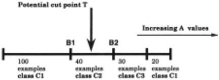
Figure 1: A potential within-class cut point.
be the proportion of examples inS that have class Ci . The class entropy of a subset S is defined as:
When the logarithm base is 2, Ent( S) measures the amount of information needed, in bits, to specify the classes inS. To evaluate the resulting class entropy after a set S is partitioned into two sets 51 and S2, we take the weighted average of their resulting class entropies:
Definition 1: For an example setS, an attribute A, and a cut value T : Let S1 C S be the subset of examples in S with A values ~ T and S2 = S - S1· The class information entropy of the partition induced by T, E(A, T; S), is defined as
A binary discretization for A is determined by selecting the cut point TA for which E( A, TA; S) is minimal amongst all the candidate cut points.
2.1 Discussion of Cut Point Selection
One of the main problems with this selection criterion is that it is relatively expensive. Although it is polynomial in com plexity, it must be evaluated N - I times for each attribute (assuming that the N examples have distinct values). Since machine learning programs are designed to work with large sets of training data, N is typically large. In the case of a nominal (or discretized) attribute, this criterion requires only a single evaluation of an r-partition, where r is the number of values of the nominal attribute. Typically, r ~ N. Indeed, experience with ID3-like algorithms confirms that they run significantly slower when continuous attributes are present.
The other objection that may be raised is that the algorithm has an inherent weakness in it that will cause it to produce "bad" cut points especially when there are more than two classes in the problem. This objection is based on the fact that the algorithm attempts to minimize the weighted average entropy of the two sets in the candidate binary partition (as shown in Equation I above) . The cut point may therefore separate examples of one class in an attempt to minimize the average entropy. Figure I illustrates this situation. Instead of falling on one of the boundaries B I or B2, the cut point may fall in between so that the average entropy of both sides is minimized. This would be undesirable since it unnecessarily separates examples of the same class, resulting in larger (and lower quality [5]) trees.
However, neither of these objections turns out to be true. Theorem I below shows that regardless of how many classes there are, and how they are distributed, the cut point will al ways occur on the boundary between two classes (see Defini tion 2 for a precise statement of what we mean by a boundary point). This is indeed a desirable property of the heuristic since it shows that the heuristic is "well-behaved" in terms of the cut points it favours. It tells us that this heuristic will never select a cut that is considered "bad" from the teleolog ical point of view. In addition, this result will also help us improve the efficiency of the algorithm without changing its function.
2.2 Cut Points Are Always on Boundaries
We show that the value TA for attribute A that minimizes the average class entropy E(A, TA; S) for a training set S must always be a value between two examples of different classes in the sequence of sorted examples. Let A( e) denote the A-value of example e E S.
Definition 2: A value T in the range of A is a boundary point iff in the sequence of examples sorted by the value of A, there exist two examples e1, e2 E S, having different classes, such that A( e 1) < T < A( e2); and there exists no other example e' E S such that A(e 1) < A(e') < A(e2) .
Theorem 1 1fT minimizes the measure E(A, T; S) , then T is a boundary point.
Corollary 1 The algorithm used by ID3 for finding a binary partition for a continuous attribute will always partition the data on a boundary point in the sequence of the examples ordered by the value of that attribute.
Proof: Follows from Theorem I and definitions.
0
The first implication of Corollary I is that it serves to sup port the usage of the entropy minimization heuristic in the context of discretization. We use the . information entropy heuristic because we know, intuitively, that it possesses some of the properties that a discrimination measure should, in principle, possess. However, that in itself does not rule out possibly undesirable situations, such as that depicted in Fig ure I. The Corollary states that "obviously bad" cuts are never favoured by the heuristic. This result serves as further formal support for using the heuristic in the context of discretization, since it tells us that the heuristic is well-behaved from the teleological point of view.
In addition, Corollary I can be used to increase the effi ciency of the algorithm without changing its effects at all. After sorting the examples by the value of the attribute A, the algorithm need only examine the b boundary points rather than all N - I candidates. Note that: k - I < b < N - I . Since typically k ~ N we expect significant computational savings to result in general. We have demonstrated significant speedups in terms of the number of potential cut points eval uated in [7] for the 103 algorithm. 103 partitions the range of a continuous-valued attribute into two intervals. Algo rithms that extract multiple intervals using a generalization of this procedure (such as the one presented in the next section) achieve higher speedups. Algorithms that search for rules rather than decision trees also spend more effort on discretiza tion. The computational speedup in the evaluation process is only a side benefit of Corollary I. Its semantic significance is our focus in this paper since it justifies our generalizing the same algorithm to generate multiple intervals rather than just two.
3 Generalizing the Algorithm
Corollary 1 also provides support for extending the algorithm to extract multiple intervals, rather than just two, in a single discretization pass. The motivation for doing this is that "better" trees are obtained 2 .
The training set is sorted once, then the algorithm is applied recursively, always selecting the best cut point. A criterion is applied to decide when to refrain from applying further binary partitioning to a given interval. The fact that only boundary points are considered makes the top-down interval derivation feasible (since the algorithm never commits to a "bad" cut at the top) and reduces computational effort as described earlier.
To properly define such an algorithm, we need to formu late a criterion for deciding when to refrain from partitioning a given set of examples. The criterion needs to be well principled and theoretically justified. Empirical tests are later used to verify that the assumptions behind the justification are appropriate.
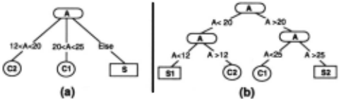
Why is the derivation of multiple ranges rather than bi nary ranges more advantageous from a tree generation per spective? Often, the "interesting" range may be an internal interval within the attribute's range. Thus, to get to such an interval, a binary-interval-at-a-time approach leads to unnec essary and excessive partitioning of the examples that are out side the interval of interest. For example, assume that for an attribute A with values in [0, 40], the subrange 12 < A ~ 20 is of interest. Assume that A's range is discretized into: {( -oo, 12), [12, 20), [20, 25), [25, oo)}. Given an algorithm, like GID3* [5], that is capable of filtering out irrelevant at tribute values, it is in principle possible to obtain the decision tree of Figure 2(a). The attribute selection algorithm decided that only two of the four available intervals are relevant. The examples outside this interval are grouped in the subset la beled S in the figure.
Using only a binary interval discretization algorithm, in order to select out these two ranges the decision tree shown in Figure 2(b) would be generated. Note that the setS is now unnecessarily partitioned into the two subsets S 1 and S2. For the first tree, the algorithm has the option of partitioning S later using some other, perhaps more appropriate, attribute. This option is no longer available in the second situation, and the choice of future attributes will be based on smaller subsets: S 1 and S2. Essentially, this leads to the same sort of problems as those caused by the irrelevant values problem discussed in [2; 5]. The details of how GID3* deals with this problem and how only a subset of the values are branched on is beyond the scope of this paper (see [5] for details.)
3.1 To Cut or not to Cut? That is the Question
Given the setS and a potential binary partition, ?rT, specified on S by the given cut value T of attribute A, we need to decide whether or not to accept the partition. This problem is naturally formulated as a binary decision problem: accept or reject ?rT. Let HT be the hypothesis that ?rT induces if it were accepted. That is, HT is the classifier that tests the value of A against T and then classifies examples that have value less than T according to the examples in E for which A-value < T . Similarly, let NT represent the null hypothesis; that is the hypothesis that would result if ?rT were rejected. Thus NT would classify all examples according to the classes in E without examining the value of A. Since accept or reject are the only possible actions, one of them must be the correct choice for this situation; the other is incorrect. Of course we have no way of directly deciding which is correct.
2 0ne tree being "better" that another in this context means that it is smaller in size and that its (empirically estimated) error rate is lower. In [4] we address the meaning of "better" more formally. See [5] for further details.
Let dA be the decision to accept the partition ?rT, and let dR represent rejecting it. The set of possible decisions in this situation is D = {dA, dR} and we have a binary decision problem to solve. If we assign a cost to our taking the wrong decision, then the expected cost associated with a decision rule that selects between { dA, dR} is expected to have cost:
where c11 and c22 represent the costs of making the correct choice, and c12 and c21 are the costs of making the wrong decision. This is the expected Bayes risk associated with whatever decision rule is being used to select one of { dA, dR}· The Bayes decision criterion, calls for selecting the decision rule that minimizes the expected cost.
Since we do not know what values to assign to c12 and c21 . we resort to the uniform error cost assignment. If we let en = c22 = 0 and let c12 = c21 = 1, then mini mizing the Bayes risk reduces to a decision rule known as Probability-of-ErrorCriterion (PEC) [ 12] which calls for min imizing the probability of making the "wrong" decision. Sub sequently, it can be shown via a simple derivation [ 12] that the Bayes decision criterion reduces to adopting the decision rule which, given data setS, selects the hypothesis HT for which Prob{HTIS} is maximum among the competing hypotheses [12]. We refer to this decision criterion as the Bayesian De cision Strategy. This strategy is also known as the maximum a posteriori (MAP) criterion [12], which in turn is equivalent to PEC.
For our decision problem, the Bayesian decision strategy (as well as MAP and PEC) calls for selecting the decision d E D that corresponds to the hypothesis with the maximal probability given a data set S: thus we should choose dA if and only if Prob{HTIS} > Prob{NTIS}. If we had a way of determining the above two probabilities our problem would be solved: simply choose the hypothesis that has the higher probability given the data, and Bayesian decision the ory guarantees that this is the best (minimum risk) strategy. Unfortunately, there is no easy way to compute these probabil ities directly. However, we shall adopt an approach that will allow us to indirectly estimate which probability is greater.
3.2 The Minimum Description Length Principle
The minimum description length of an object is defined to be the minimum number of bits required to uniquely specify that object out of the universe of all objects.
We shall show that in the case of our decision problem, we can employ the Minimum Description Length Principle (MDLP) to make a guess at the hypothesis with the higher probability, given a fixed set of examples. The MDLP is a general principle that is intended to encode the natu ral bias in science towards simpler theories that explain the same body of data. The MDLP was originally introduced by Rissanen [17] and has later been adopted by others [14; 18] for use in induction. We define it as defined in [14] :
Definition 3: Given a set of competing hypotheses and a set of data S, the minimum description length principle (MDLP) calls for selecting the hypothesis HT for which MLength(HT) + MLength(SIHT) is minimal among the set of hypotheses. MLength(HT) denotes the length of the minimal possible encoding of HT, while MLength(SIHT) is the length of the minimal encoding of the data given the hypothesis.
For convenience, we assume lengths are measured in bits. The encoding of the data given the hypothesis may be thought of as encoding the data points that are the "exceptions" to the hypothesis HT. If HT fits the data exactly, then the latter term goes to zero.
The MDLP principle is not necessarily calling for some thing different from the decision criteria discussed earlier. It can be easily shown that the MDLP and the Bayesian risk minimization strategy (under the assumption of uniform error cost) are theoretically related to each other. For lack of space we omit the derivation which simply consists of expanding the expression for the number of bits needed to specify the hypothesis H given the data S: -log2(Prob{HIS} ), using Bayes' rule. The final expression obtained is equivalent to the MDLP. This will serve as motivation for adopting the MDLP since it reduces the arbitrariness of our adopting it over some other heuristic for deciding when to refrain from further partitioning.
Based on our earlier arguments, if we had a way of finding the true minimal encoding length of hypotheses and of the data given a hypothesis, then employing the MDLP for selecting one of a set of competing hypotheses leads to choosing the hypothesis with the maximum a posteriori probability (given the data). Consequently, this is equivalent to the PEC decision criterion. This means that the selected hypothesis will be the one which minimizes the probability of having made the wrong selection decision. However, in the physical world we do not have access to the probability distributions. Hence, the MDLP is used as an estimate of cost, or a heuristic, for distinguishing between hypotheses.
3.3 Applying the MDLP: A Coding Problem
Now the problem at hand is a coding problem. In our case, the decision problem is relatively simple. The set of competing hypotheses contains exactly two elements: {HT, NT} . We shall employ the formulation used by Quinlan and Rivest [14] where they used the MDLP in attribute selection in an attempt to generate compact decision trees (see [ 18] for a commentary on [14]). In our case, the problem is fortunately simpler.
Using the formulation of [14], the problem that needs to be solved is a communication problem. The goal is to communicate a method (classifier), that will enable the receiver to determine the class labels of the examples in the set. It is assumed that a sender has the entire set of training examples, while a receiver has the examples without their class labels. The sender needs to convey the proper class labeling of the ex ample set to the receiver. The sender must essentially choose the shortest description for specifying the classes.
Coding the Null Theory NT : In the case of NT, the sender must simply transmit the classes of the examples in S in sequence. The sender sends N messages, each being a coded class label (where N = lSI). To encode the classes of the examples inS, we may use an optimal (e.g. Huffman coding) algorithm [16] to produce code optimized for average code length. Since we have to transmit the class for each example in the setS, multiplying the average code length l by N gives us the total cost of transmitting the classes of the examples in S . In addition, one needs to transmit the "code book" to be used in decoding the classes. Transmitting the code book consists of sending the code word associated with each class. Hence, if there are k classes the length of the code book is estimated by (k · l). Note that k is a constant that does not grow with N, so the cost of the code book is a small constant overhead.
Coding the Partition HT : The cut point chosen to parti tion the examples must be specified by the sender followed by an encoding of the classes in each of the two subsets. Speci fying the cut value costs log 2 (N - 1) bits since we need only specify one of theN - I examples in the sequence which the cut value falls just before (or after).
The classifier HT corresponding to the binary partition, 7rT, partitions the set S into subsets S1 and S2. What the sender must transmit, then, is a specification of the cut point followed by the sequence of classes in sl followed by the classes in S2. Again, all we are interested in determining is the minimal average length code for the classes in sl and s2 as we did in the case of encoding the classes inS. Let l1 and lz be the minimal average code lengths (in bits) for the classes in S1 and S2 respectively. The cost of transmitting HT along with the data given HT is
We also need to transmit the code books for the respective codingschosen for the classes in S1 and S2. Unlike the case of transmitting S where we knew that all k classes are present, in this case we must inform the receiver which subset of classes is present in each of the two subsets S1 and S2, and then send the respective code books. Since we know that our partition is non-trivial, i.e. S1 =f. S2 =f. 0, we know that S1 can have any one of 2.1: - 1 possible subsets of the k classes. Using a lengthy derivation, it can be shown that
is the number of possible partitions out of which we need to specify one. Hence we need 1og2 (�o~:) bits. Note that log2 (�o~:)< 2log2 (2.1:- 1) < 2k.
3.4 The Decision Criterion
In our quest for the "correct" decision regarding whether or not to partition a given subset further, we appealed to the MDLP.
| DataSet | name | examples | attributes | classes |
|---|---|---|---|---|
| Faulty operation data from the JPL Deep Space Network antenna controller | DSN | 258 | 12 | 5 |
| Problems m a reacttve ton etcnmg process tKihJ m semtconouctor manu- facturin~ from Hu~hes Aircraft Company | SRCl | 94 | 8 | 4 |
| The waveform domain described in [1] | WVFRM | 150 | 21 | 3 |
| uata ootameo trom a response sunace or multtple response vanao1es m a set of wafer etchin~ experiments conducted at Hu~hes | RSMl | 300 | 3 | 35 |
| RSMl with classes mapped to only two values: "good" and "bad" | RSM2 | 300 | 3 | 2 |
| Publicly available heart disease medical data from an institute in Cleveland | HEART | 303 | 13 | 2 |
| The glass types data from the USA Forensic Science Service | GLASS | 214 | 9 | 6 |
| The famous iris classification data used by R.A. Fisher (1936) | IRIS | 150 | 4 | 3 |
| The echocardiogramdata of heart diseases from the Reed Institute of Miami | ECG | 132 | 9 | 2 |
In turn, this gave us a coding problem to solve. The solution is readily available from information theory, c.f. Huffman coding. However, we are not interested in the actual minimal code itself. The only thing we need to know is the average length of the minimal code. The following theorem gives us this information directly and in the general case.
Theorem 2 Given a source of messages s with entropy Ent(s), for any f > 0, there exists an optimal encoding of the messages of s such that the average message code length l, in bits, is such that En~s) ~ l < Ent(s) +f.
Proof: See Shannon's Noiseless Coding Theorem in [9]. 0 Note that this theorem requires that the entropy Ent(S) be defined using logarithms to the base 2. In the case of our simple communication problem, the source of messages is the sender and the messages are the encoded classes. Theorem 2 tells us, that "we can bring the average code word length l as close as we please to the entropy" of the source [9].
Let l be the average length of the code chosen to represent the classes in S. Similarly, l1 and h are the corresponding average code lengths for S1 and S2. Putting all the derived costs together we obtain:
The MDLP prescribes accepting the partition iff Cost( HT) < Cost( NT). Examine the condition under which (Cost( NT) - Cost( HT)] > 0:
Now recall that the information gain of a cut point is
The above inequality, after dividing through by N, reduces to
where A( A, T; S) =
We are now ready to state our decision criterion for accept ing or rejecting a given partition based on the MDLP:
MDLPC Criterion: The partition induced by a cut point T for a set S of N examples is accepted iff G . (A T· S) log2 (N- 1) A( A, T; S) am ' , > N + N and it is rejected otherwise.
Note that the quantities required to evaluate this criterion, namely the information entropy of S, S1, and S2 are com puted by the cut point selection algorithm as part of cut point evaluation.
4 Empirical Evaluation
We compare four different decision strategies for deciding whether or not to accept a partition. For each data set used, we ran four variations of the algorithm using each of the following criteria:
- Never Cut: the original binary interval algorithm.
- Always Cut: always accept a cut unless all examples have the same class or the same value for the attribute.
- Random Cut: accept or reject randomly based on flipping a fair coin.
- MDLP Cut: the derived MDLPC criterion.
The first three strategies represent simple alternative decision strategies that also cover the continuum of decision strategies since the first two are the two extrema.
We used the data sets described in Table 1. Some of these were obtained from the U.C. Irvine Machine Learning Repos itory and others from our own industrial applications of ma chine learning described in [10]. The data sets represent a mixture of characteristics ranging from few classes with many attributes to many classes with few attributes.
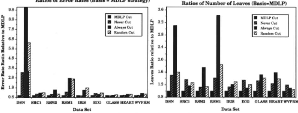
For each data set, we randomly sampled a training subset and used the rest of the set for testing. For each data set we repeated the sampling procedure followed by generating the tree and testing it 10 times. The results reported are in terms of the average number of leaves and percentage error rate on classifying the test sets. The results are shown in Figure 3. Note that there is no difference between the tree generated by GID3* under the Never Cut strategy and the tree generated by the ID3 algorithm. Thus, those columns in the charts may be taken to reflect ID3's performance. For ease of compar ison, we plot the results in terms of ratios of error rate and number of leaves of the various cut strategies to the MDLP Cut strategy. Note that the improvements are generally sig nificant. The data set RSMI proved a little problematic for the MDLPC. One possible reason is that the number of classes is large and the number of training examples is probably not sufficient to make the recommendations of the MDLPC crite rion meaningful. Note that this hypothesis is consistent with the fact that performance dramatically improved for the set RSM2 which is the same data set but with only two classes.
5 Conclusion
We have presented results regarding continuous-valued at tribute discretization using the information entropy minimiza tion heuristic. The results point out desirable behavior on the part of the heuristic which in turn serves as further theoreti cal support for the merit of the information entropy heuristic. In addition, the efficiency of the cut point selection heuristic can be increased without changing the final outcome of the algorithm in any way. Classification learning algorithms that use the information entropy minimization heuristic for select ing cut points can benefit from these results. We also used the results as · a basis for generalizing the algorithm to mul tiple interval discretization. We derive a decision criterion based on information and decision theoretic notions to decide whether to split a given interval further. Coupled with formal arguments supporting this criterion, we presented empirical results showing that multiple interval discretization algorithm indeed allows us to construct better decision trees from the same data.
Acknowledgments
We thank Hughes Microelectronics Center for support in the form of an unrestricted research grant. The work described in this paper was carried out in part by the Jet Propulsion Laboratory, California Insti tute of Technology, under a contract with the National Aeronautics and Space Administration.
@inproceedings{ijcai1993p141,
  title     = {Multi-Interval Discretization of Continuous-Valued Attributes for Classification Learning},
  author    = {Fayyad, Usama M. and Irani, Keki B.},
  booktitle = {Proceedings of the Thirteenth International Joint Conference on
               Artificial Intelligence, {IJCAI-93}},
  publisher = {International Joint Conferences on Artificial Intelligence},
  editor    = {Ruzena Bajcsy},
  pages     = {1022--1028},
  year      = {1993},
  note      = {Machine Learning},
  url       = {https://ijcai.org/proceedings/1993/141},
}
TY - CPAPER TI - Multi-Interval Discretization of Continuous-Valued Attributes for Classification Learning AU - Fayyad, Usama M. AU - Irani, Keki B. T2 - Proceedings of the Thirteenth International Joint Conference on Artificial Intelligence, IJCAI-93 PB - International Joint Conferences on Artificial Intelligence PY - 1993 SP - 1022 EP - 1028 UR - https://ijcai.org/proceedings/1993/141 ER -Copied
Machine-readable versions of this paper, for tools and AI agents:





