On Seeing Spaghetti: A Novel Self-Adjusting Seven Parameter Hough Space for Analyzing Flexible Extruded Objects

1. Introduction

We consider the problem of analyzing dense depth images to determine the parameters of flexible extruded objects. Our approach views such objects as being piecewise toroidal, since the torus is the simplest solid geometric object whose gener­ ating axis exhibits curvature. This is justified by our observa­ tion that many piecewise sections of flexible extruded objects have co-planar spines, either because they are easy to manu­ facture that way, or because they represent a minimum energy configuration (these reasons are often equivalent). However, a torus is an object with seven free parameters: three of position, two of orientation, one of size, and one of relative

Rick Kjeldsen

Exploratory Computer Vision Group IBM Thomas J. Watson Research Center P.O. Box 704 Yorktown Heights, NY 10598 fcmk@watson.ibm.com

"thickness". This pushes the limits of the current state of the art in parsing high-degree parametric object models, particu­ larly since the parameters of position and size are potentially unbounded, especially for objects that are nearly cylindrical.

Following what might be called the principle of least variability, we first recover the thickness parameter, since among all seven it is the one parameter most likely to be constant across the toroidal pieces. The method exploits a novel but efficient algorithmic interpretation of a result in differential geometry called Meusnier's theorem. Then, using the knowledge gained from deriving the thickness, we recover the next most well-behaved parameters, the orientation and size. These are computed simultaneously and in a manner that compensates for the ill-conditioning of orientation estimates when size is large. Lastly, using knowledge of both thickness and size, we recover the position of the local toroidal section, again automatically compensating for the ill-conditioning of large and/or nearly straight objects.

The significance of the work rests on its two principal results: the elegance and speed of the thickness-finding trans­ form (reviewed only briefly here, for more details see [Kender and Kjeldsen, 1990], and the novel way in which the parameter space structure decomposes a difficult seven-dimensional problem so that ill-conditioned hypotheses cluster together for easy detection and removal. The work as a whole is applicable in vision systems wherever depth and surface orientation (however sparse) are obtainable, particularly for those cases where object boundaries are occluded, and where contour­ based methods therefore fail.

1.1. The Torus in Brief

We adopt the terminology ofDoCarmo [1976], and review the results on tori that we will exploit.

A torus is a solid of revolution formed by a generating circle ("minor circle") of radius r being swept in a circle of revolution ("major circle") of radius a (Note that we have reversed the sense of r & a from DoCarmo ). Generally speak­ ing, we will assume that r<a, that is, that the "donut" has a "hole". This constraint will be exploited in the decomposition of the parameter spaces.

Surface properties are best represented in the framework of the following parameterization, which identifies the center of the torus (and hence, the center of the major circle) with the center of a cylindrical coordinate system, making a to be cylindrical radius and v as cylindrical angle; the axis of the torus becomes the remaining coordinate z. We parameterize the surface of the minor circle by the angle u; unlike the angle v, its origin is critical, and is set to equal 0 when it is most distant from the torus center. The locus of points with a given v lie on a "meridian". The locus of points with a given u lie on a "parallel".

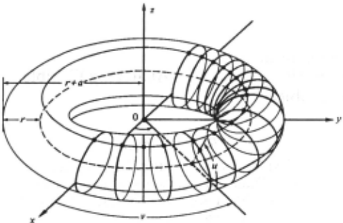
As with any other regular surface, each point of the torus has two principal curvatures, with directions of principal cur­ vature that are perpendicular to each other. Every point has one positive curvature, k1, which is oriented along the merid­ ian. The other curvature of the point, k2, is more elaborate, although it is always oriented along the parallel. k2 is 0 at the "top" and "bottom" parallels of the torus, where the surface is locally cylindrical. It attains its extreme positive value at the "outermost" parallel, and its extreme negative value at the "innermost" parallel. We note and will heavily exploit the observation that the largest positive curvature at any point is always the value of k1.

We will adopt the following notation. A point on the torus is denoted as Pi; it is considered to be vector in three space. We will abbreviate the vector Pi-Pj as Pij· Likewise, we will refer to the unit normal vector of the surface at Pi as Ni, and a similar comment applies to vectors of the formNij. Note that the values of the points and the normals are available as input data, measured in the coordinate system of the imaging appa­ ratus. We will often refer to the "translated" points Ti =Pi - rNi ; if the r is the true minor radius, then Ti = Si, that is a point on the torus spine.

2. Computing Minor Radius

It is not hard to show that when computing the parameters of a two-dimensional surface in three space, the information that a point is on the surface can be used to fix one parameter, and the information that a given vector is the normal to the surface at a point can be used to fix two parameters. (Analo­ gous statements can be made about curvature, but we avoid curvature information because of its intrinsic susceptibility to noise.) Thus, a sphere is uniquely determined by four points, or, more simply, by two points and the normal at one of them.

Thus, two points and their normals are insufficient to uniquely determine a torus, since they fix only six parameters. How­ ever, three points and their normals in general overdetermine the torus in the following way. There must exist a local space circle that serves as the torus spine, and it must be equidistant from all three points (this common distance is the value of r). But, in addition, this space circle must have the property that at the point of closest approach to each of the Pi, the tangent to the space circle must be perpendicular to the corresponding Ni. It is the need for some means to guarantee this tangent property tha~ leads to the following observations and construc­ tions.

We select a distinguished point Pi; without loss of gener­ ality assume that it is the point Pl. We then construct all the space circles through the translated point T1 whose tangents at T1 are perpendicular to N1, and that also pass through a second translated point, call it rz. There is a one degree of freedom family of such circles, and they all lie on the surface of a sphere. That such a conl'!truction is possible can be seen both geometrically and algebraically; it is also a special case of the theorem of Meusnier. (Meusnier's theorem states that if a set of planes are drawn through a tangent to a surface in a non -zero curvature direction, then the osculating circles of the intersections with the surface lie upon a sphere [Struik, 1961 ].)

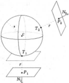
Geometrically, we consider T1 to be the south pole of a sphere whose north-south axis is collinear with N1. The size of the sphere is deter­ mined by Tz, Call this sphere the supporting sphere. Any circle (great or little) that passes through T1 and Tz now L ____________________ ,/ also has its local tangent at T1 perpendicular toN1. /'-I-- 1 ~ Algebraically, we can look for the size of the support sphere, s; since .

constrained to lie along the direction of the N1, the center is given by C=Tl +sN1. Both T1 and Tzlie on a common sphere if their distances from the center are equal. This is captured by equating the norms of their relative position vectors, giving in vector form the equation of the plane of their perpendicular bisectors: IC-Tli=IC-Tzl. Expanding, we find that sz(r), that is, the size of the support sphere needed to accommodate T2 ,is a function of r.

Note, however, that the local tangent at T2 is not necessar­ ily perpendicular to Nz. Worse, T3 may not even lie on the support sphere at all.

We remedy this second defect first, by constructing with T1 and T3 the same sort of support sphere as was constructed with T1 and Tz. What results is a symmetric relationship,

which expresses the size of the support sphere which would not only accommodate T3, but which would also allow us to draw a one-dimensional family of circles through T1 and T3 whose local tangents at Tl are perpendicular N1.

Now note that if S2(7)=S3(7), for whatever 7, the support spheres must be coincident, since they are both defined relative to P1, and all three Ti lie upon it. Basically, equating S2(7)=S3(7) will find those 7 that allow a solution to the now overdetermined problem of finding a sphere that passes thr?ugh three points and attains a specified normal at a given pomt (here, the south pole). Equating sz(r)=S3(7) gives a dr . . A 2 qua atic m 7; 7 +B7+C = 0, where

This equation will have at most two solutions for the value of 7, and they are easily obtainable by the quadratic formula. Since they are based on T1 being the south pole, call them 71,1 and 71,2· We still have to address the need for T2 and T3 to satisfy their tangent condition, however. We do this in a completely symmetric fashion, by finding two more support sphere systems, first by considering T2 a south pole, and then T3. The quadratic equations in 7 that result are derived by inspection by permuting the indices of the Pi and Ni.

From T2 as south pole we get two more candidates for the value of 7, 72,1 and 72,2, and from T3 we get 73,1 and 73,2· This wou~d. appear to call for the calculation of 24 inner products, but 1t 1s easy to show that any two of these three quadratics have four inner products in common; thus, there is a total of only 12 innerproducts.

We now have three pairs of candidate 7 values. Let us define a consensus 7 to be any 7ij that satisfies

There may be zero, one, or two consensus 7. They can be accumulated and filtered in the usual Hough way using a one-dimensional parameter space. We note several properties of this consensus algorithm.

The values of 7 are derived by independently solving three quadratics in 15 image observables (three for each point Pi, and two for each unit normal Ni). The virtue of this method is that despite the non-linearities that would result when vari­ ables are eliminated, the method does not require any iterative root finding. Nor does it suffer from the attendant problems of choosing starting values, guaranteeing convergence or tracking multiple roots. '

Enlisting the aid of IBM's proprietary symbolic math system Scratchpad III [Jenks et al., 1986], we were able to show that the transform always produced one consensus value for 7, corresponding to the true minor radius of the torus and '

that if a second consensus existed, it was always easily distin­ guishable by its sign and/or magnitude from the true consensus 7, which is always the smallest positive radius of curvature.

Further, the analysis suggested several intriguing exam­ ples of what should probably be called anti-tori. The most straightforward example is what happens when two of the data points are on a meridian, and the third is on the innermost parallel. The transform properly returns two consensus: one is 7, and the other is -1,.-ta-r), the value of kz at the "innermost" parallel. What the transform "sees" is an anti-torus whose thickness is equal to the torus' hole, and whose hole is equal to the torus' thickness. That is, it interprets the data to be lying o~ the negative _image of an ~nti-torus, whose axis is perpen­ dicular to the g1Ven torus, w1th the torus and anti-torus inter­ locking: much like confusing the impression in plaster of a face with the face itself.

3. Computing Orientation (and Major Radius)

Following the principle of least variability, we next re­ cover orientation by examining the spine points produced by our ~ndi~ate 7. Orientation is a naturally bounded quantity, and 1s easlly represented as a point on the sm;face of the upper Gaussian hemisphere (mathematically, on r).

The approach is straight forward: given a candidate r we form the spine points Si =Pi - rNi from the pixels suppo;ting r, and determine the orientation of the plane on which they lie. The direction of the plane's normal is easy to compute: simply take the normalized unit vector of the following cross product (or any of its variants obtained by permuting the Si):

However, this orientation is ill-conditioned when the spine points are nearly co-linear, which occurs when a is large. Using derivatives, it is not hard to show that small changes of S2 in a direction perpendicular to this plane have an effect on the plane's or~entation that is roughly proportional to the major radlUs, a. Th1s suggests that the computation for orientation should be accompanied by the computation of a, so that orientation can be "weighted" inversely by a somehow.

Rather than use a as a pure parameter space voting weight, we note the following. The value of a eventually has to be recovered anyway, and if it disappears into a weighted sum it is not recoverable. Instead, we scale the unit orientation vector by dividing it by a. The parameter space now becomes the interior of the upper Gaussian hemisphere, which is three di~ensional, and the values of a are recoverable simply by taking each vector's length. More importantly, orientations accompanied by high a cluster near the origin, where they are easy to detect and remove. Conversely, other orientations receive parameter space representation proportional to their certainty, since they are proportionately distant from the hemi­ sphere center.

This parameter space has two other advantages. First, it uses the interior of what would otherwise be a very inefficient use of three-space, thus obviating the need to cleverly tessel­ late the surface of the Gaussian sphere. Secondly, points that cluster at its origin can immediately be considered evidence of cylindrical objects in the image (which have no orientation and infinite a).

Since the orientation and a spaces are now combined, the computation of the resulting parameter point (the scaled ori­ entation vector) can also be combined; it is not necessary to actually plot the spine circle or calculate its center. By means of a three-space geometric construction related to the planar "Law of Sines" for circles, it can be shown that the scaled vector is directly given by the following (or by any of its variants obtained by permuting the Si):

where

4. Computing Center

What remains are the three most difficult parameters, the center parameters, which are potentially unbounded and highly sensitive to the value of a. Local tori with small curvature have distant centers which are difficult to compute accurately. Since triangulation error of the center is also roughly proportional to a, this final space computes and accu­ mulates vectors to the center point, scaled again by a. In effect, this measures each center in units of major radius, thus relative error is nearly constant. It is not hard to show that this space is now bounded, since for local tori with large a, their center must be about a units from the image origin, otherwise they would not fall within the image. Thus, most tori have centers within one unit from the origin. The upper limit of this space is determined by small tori at the image edge; since a is bounded by r, and r is bounded by physical considerations, this limit is calculable directly.

We note that although many tori might map to the same scaled vector, they have already been classified and separated by the value of a in the prior parameter space. Thus, the nesting of these spaces is critical both for adjustment to error, and for disambiguation of results.

The computation is straightforward but a bit messy (how­ ever, it is again invariant to the permutation of the Si):

where

5. System Considerations

In practice, the above method relies on the ability to pick "good" triples of points Pi. Additionally, the performance and behavior of the method can be enhanced by simple "sanity checks" on computed intermediate results. Lastly, the orienta­ tion space can be improved by a judicious choice of "offset" for the scaled orientation vector. We handle these in tum.

Picking good triples is determined by enforcing a mini­ mum and maximum distance between image points Pi; we call this distance the "radius of coherence" (ROC). If the ROC is too small, accuracy suffers due to small triangulation baseline; too large, and most triples do not lie on the same torus. For the minor radius space, it can be set in accordance with the expected range of minor radii, which can be determined from the imaging parameters. Empirically, we have found that a wide range between minimum and maximum ROC works well for minor r. The two other spaces have similar considerations, however the range between minimum and maximum ROC must be rather narrow or the system becomes overwhelmed with noise hypotheses. Fortunately, experience shows that a narrow range of ROC about r works very well for a large range of torus shapes.

Sanity checks are inexpensive checks on the data before it is used in a parameter transform. Our sanity checks are of the following form. In computing r, no points in a planar neigh­ borhood are used; they are easy to detect, since they have very small and equal principal curvatures. Nor are points near a depth discontinuity used, as the surface approximations be­ come inaccurate there. Further, degenerate quadratics (with A=O or with imaginary roots) are ignored . In computing orientations and centers, spine points within a pixel of each other are ignored. These checks take a minute percentage of the computation times, but reduce the noise in parameter space dramatically.

In practice, the scaling of orientation vectors by Va results in vectors too tightly clustered around the origin. This is because any torus large enough to be seen in the image as a torus will have a major radius of at least eight pixels, approxi­ mately. Thus, all the activity in the space happens in a hemi­ sphere of radius ¥8; this uses less than 1% of the space. If a lower bound on a is known (and it usually can be approxi­ mated), then the scaling function should be of the form bJta+c), with c serving to shift small values of a closer to the surface of the hemisphere. Heuristic choices of constants based on expected torus and image sizes can be selected; one good one maps the smallest torus onto the surface of the hemisphere, and the largest torus that can be fully seen (a=64, assuming a range image of size 256) into the midpoint of the hemisphere; the scaling function becomes 5~a+48).

6. System Description

We briefly survey the complete system of which this transform is a part, highlighting those aspects most germane to our results. A more complete description can be found in [Kjeldsen et al., 1989).

Recognition is structured as a hierarchy of layered and concurrent parameter transforms [Ballard, 1981 )[Sabbah, 1985). Each transform examines input data or previously established features and accumulates evidence for new feature hypotheses in an associated parameter space. Compatibility relations accumulate evidence for or against a hypothesis on the basis of peer hypotheses. A large number of hypotheses are typically generated. The evidence for and against each is integrated using an iterative refinement process in a dynami­ cally constructed constraint satisfaction network [Feldman & Ballard, 1981).

Each parameter space is instantiated as a subnetwork where nodes correspond to hypotheses. The links in the net­ work are (1) bottom-up connections, representing support from input data, and (2) lateral links between hypotheses. The former links can be thought of as votes generated by the parameter transforms [Hough, 1962]. The latter links, gener­ ated by the compatibility relations, can be inhibitory, or exci­ tatory. For example, surface hypotheses generated from the same pixels are connected by an inhibitory link, because they represent conflicting interpretations of the same data.

Evidence integration works as follows. Each node i com­ putes an activation level Ui representing a confidence level in the corresponding feature. At each iterative step t, the activa­ tion level of a node, denoted by Ui(t), is computed as

where /i represents bottom-up support for feature i, and the summation embodies the collective inhibition and excitation of conflicting and cooperating hypotheses j. The weight factor Wij is negative when hypothesis j conflicts with hypothesis i and positive when hypothesis j is supporting i. Di is a decay term that suppresses spurious hypotheses with little support, and helps insure stability.

A unit "survives" iteration when it has sufficient u; and insignificant inhibition. It is then passed to the next parameter transform in order to create hypotheses in higher-level spaces. Units also feed-back to their component features in lower­ level spaces and to consistent hypotheses in parallel spaces. Thus, surviving features form stable coalitions which repre­ sent globally consistent interpretations of the scene.

Additional features are added to the system by defining parameter transforms and compatibility relations which work within a well defined 1/0 structure. These generally make use of techniques described in [Califano, 1988) and [Califano et al., 1988]. Our first transform takes triples of data points and returns values of ron the basis of the consensus in Eq 2a. The second transform takes triples of the data points that support a surviving r hypothesis, and returns the parameters of the scaled vector of section 3. Finally data points supporting surviving orientation/major radii are used as described in section 4. The current system contains 21 parameter transforms for various features.

The lowest level of the system extract local features such

as surface approximations or depth discon­ tinuities from the data for use by the parame­ ter transforms. The local features impor­ tant to this work use bicubic interpolations to obtain the least mean square error fit to dense depth data, then computes di­ rectly from the poly­ nomial coefficients of the

I

approximation Fig. 5: Points voting for minor radius.

both the surface gradient vector, and the directions and amounts of principal surface curvature [Sabbah & Bolle, 1986). Experiments comparing computed values with known true values indicate that over a wide range of imagery and circumstance the inaccuracy of the approximations is no more that 5% from the ideal.

7. Results

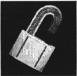
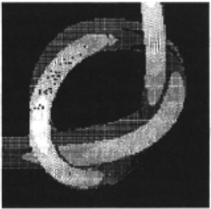
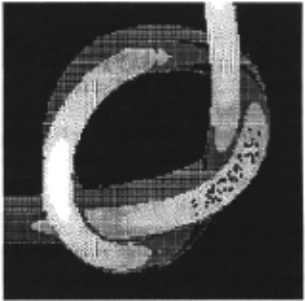
The torus extraction transforms have been run on about a dozen images. We will present two of the more interesting cases. The first is a depth map generated from a CSG repre­ sentation of a padlock (figure 3). The image contains a single torus segment, as well as several other surfaces. The second image is an actual range image of a knotted length of cable (figure 4). The cable forms a continuously varying tube of constant cross section, which can be reasonably approximated as piecewise toroidal.

In both cases we used only a small percentage of the possible triples within the ROC; the percentage was large enough to give reasonable coverage but small enough to give acceptable running times. Additionally, hypotheses receiving votes from fewer than 20 triples were not instantiated. Since many noise hypotheses receive just a few votes, this pruning helped cut down on the time and memory needed to support them.

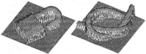
Fig. 4: Depth map of knot.

Figure 3 shows a 64x64 plot of the 256x256 depth map of the lock. Surface approximations were taken using a 5x5 window around each point. After the sanity checks, only the points hilighted in the dithered image in figure 5 were passed to the minor radius parameter transform. ROC was 9 to 10, and 50% of the possible triples were used. 10 hypotheses received votes from more than 20 triples, and so took part in iteration. After 11 iteration steps a single hypothesis of 16.5 for r survived, which corresponds closely to the apparent

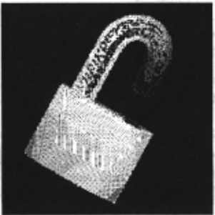
radius of the hasp.

Figure 6 shows the points which sup­ ported the winning r. To find the orienta­ tion/major radius, ROC was set to range from 15 to 16 (ap­ proximately r) and 50% of the triples formed from the spine points were used. 102 hypotheses re­ ceived sufficient support to be instantiated.

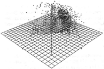
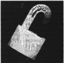
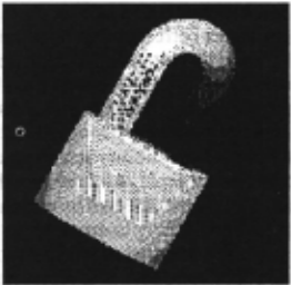
Figure 7 shows the hypotheses receiving votes plotted in utes. Generating votes for location space took 3 minutes. In 3-space (it does not show the number of votes each received). all, 30 iterations were needed to prune down the hypotheses. You can make out the hemispherical outlines of the parameter Total time for all iteration was roughly 3 minutes, including a

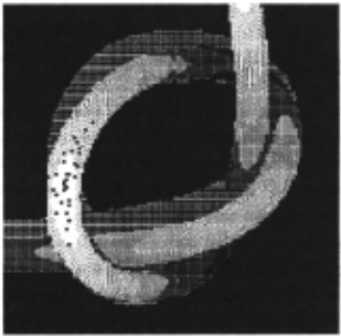
space, as well as a distinct cluster of hypotheses in the -x +y rather elaborate trace of system status. +z quadrant. Two hypotheses survived after iteration. The points supporting them are shown in figures 8 and 9. The first 7.2. Knot captured the orientation of the torus forming the top of the hasp The second image is a range image of a knot of coax cable as closely as we were able to measure it ourselves. The major (figure 4) taken using a laser triangulation range finder [Techradius was captured as accurately as the parameter space nical Arts, 1986]. ROC was the range 4 to 5, hit rate was 50%. resolution (bucket size) would allow (actual a=34, computed Figure 10 shows the points supporting the winning (and cora=37). The second surviving orientation hypothesis "found" rect, as far as we can measure) minor radius hypothesis. a very large diameter torus (a=523) on the straight segment of easily be adjusted to eliminate such misinterpretations.

Both orientation hypotheses now voted into location space. The same ROC and hit rate were used. The cylindrical segment was not able to find any consistent location, and therefore the results to within one bucket of available resolution.

These points were passed thru the orientation/major radius the hasp. As we mentioned in section 3, it is possible to parameter transform. Despite the lack of distinct peaks in the eliminate hypotheses of very large radius, that is near-cylin- histogram of votes (figure 11), the iterative refinement was ders by discarding those very close to the origin of the parame- able to find three distinct clusters, representing competing ter space. Since the length of the parameter vector of the torus hypotheses of orientation from different areas of the knot. The on top of the hasp is .65, and the length of the parameter vector strongest hypothesis in each cluster survived iteration. The for the torus found on the cylinder was .1, the cutoff could points supporting them are shown in figures 13, 14 and 15. The light coverage is due to the low hit ratios (10%) we had to use. The low hit rate also appears responsible for some regions of the knot not being covered by any hypotheses.

Figure 12 shows a histogram of the votes the three oriencreated no hypotheses strong enough to be considered. The tation hypotheses generated in location space. One peak was actual torus created 25 hypotheses. Only one survived itera- generated by the segment in fig.15, and the other peak is an tion. The surviving center was (30 67.5 -30), with the actual overlap of the votes from both fig. 13 and fig. 14. The two center at approximately (31 66 -32). Thus, the system found locations which survived iteration correspond well to the center points we expected from those torus segments.

These runs were done on a Symbolics 3650. With the Running times were somewhat better than those for the parameters set as described the entire recognition took roughly lock test case, except for the time to generate votes for orien70 minutes. Computing the surface approximations took 10 tation hypotheses. Here the continuously varying curve ereminutes. Generating the votes for minor r space took 30 ated a very large number of noise hypotheses, and very wide minutes. Generating votes for orientation space took 25 minin the histogram of votes. With the 10% hit rate used here, roughly 4000 hypotheses were created. Unking them [Califano et al., 1988] A. Califano, R.M. Bolle, and R.W. took well over an hour. With somewhat higher hit rates, 21000 Taylor, "Generalized neighborhoods: A new approach to hypotheses were created. Many hours were needed to create complex feature extraction," IEEE Conf. on Comp. Vision and link them. and Pattern Recognition, Nov. 1988.

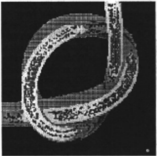
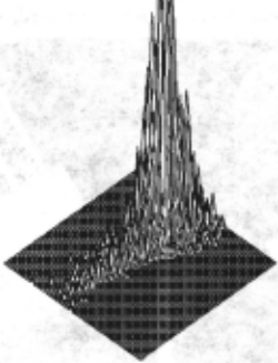
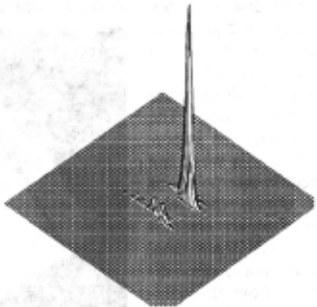
Fig. 12: Pixels supporting winning location.

7.3. Discussion

These experiments demonstrate the ability to break a con­ tinuously varying curve into piecewise toroidal segments, to deal with non-toroidal surfaces and cylinderical segments. We hope that speeding the implementation and a future port to faster hardware will improve the coverage, but these results are very promising.

System parameters must currently be adjusted for each image. An initial setting generally gives either impossibly long running times, due to the number of hypotheses created, or poor coverage of points supporting the winning hypotheses. The latter makes recognition in subsequent parameter spaces difficult. ROC and hit rate can generally be adjusted for good coverage in reasonable time, but it takes several attempts. A faster implementation would allow us to use all triples and a wider ROC, especially in minor radius space. We believe this would almost eliminate the need to tune system parameters.

Acknowledgments

This work was performed while the first author was par­ tially supported on sabbatical leave by IBM Hawthorne; addi­ tional support was provided by the Defense Advanced Research Projects Agency, contract N00039-84-C-0165. We thank Sanjaya Addanki, Ruud Bolle, Andrea Califano, and Rakesh Mohan for their generosity and insight. We especially are grateful to another visitor, Russell W. Taylor, for many useful discussions over donuts, and anti-donuts.