
Parallel Distributed Belief Networks That Learn
Proceedings of the Twelfth International Joint Conference on Artificial Intelligence. Qualitative Reasoning. Pages 1210-1217.
© 1991 International Joint Conferences on Artificial Intelligence
Abstract
A parallel distributed computational model for reasoning and learning is discuBBed based on a belief network paradigm. IBBues like reasoning and learning for the proposed model are discu88ed. Comparisons between our method and other methods are also given ..
- Beeri et al., July 1983]
- Catriel Beeri, Ronald Fagin, David Maier, and Mihalis Y annakakis. On the de- sirability of acyclic database schemes. Journal of the ACM, 30(3):479-513, July 1983.
- [Bourlard and Wellekens, 1990] H. Bourlard and C. J. Wellekens. Links between markov models and multi- layer perceptrons. IEEE 7ran.~. Pattern Analy1u and Machine Intelligence, to appear, 1990.
- [Cooper, 1984] G. F. Cooper. NESTOR: a computer- based medical diagnostic aid that integrates causal and probabilistic knowledge. Report HPP-8-/-../8, Stanford Univer1ity, 1984.
- Gallant, Feb 1988]
- S. I. Gallant. Connectionist expert systems. Communication.~ of the ACM, 31(2):152-169, Feb. 1988.
- [Herskovitz and Cooper, 1990] E. Herskovitz and G. F. Cooper. Kutato: An entropy-driven system from construction of probabilistic expert systems from databases. In M. Henrion and Bonissone, editors, Proc. 6th International Conf. on Uncertainty in Al Cambridge, MA., July 1990. North Holland. '
- [Jeffrey, 1957] R. Jeffrey. Contributions to the theory of inductive probability. Ph. D. the1u, Department of Philo1ophy, Princeton Univer1ity, 1957.
- [Judd, 1987] S. Judd. Learning in networks is hard. In Proc. IEEE Fird International Conf. on Neural Net- work.., volume 2, pages 685-692, San Diego, CA, Jun 1987. IEEE Press.
- [Kullback, 1968] S. Kullback. Information Theory and Statutic1. Dover Publication, Inc., New York, 1968.
- [Laskey, 1990] K. B. Laskey. Adapting connectionist learning to hayes networks. International Journal of Approzimate Rea~oning, 4:261-282, 1990.
- [Lauritzen and Spiegelhalter, 1988] S. L. Lauritzen and D. J. Spiegelhalter. Local computations with proba- bilities on graphical structures and their application to expert systems. J. R. Statut. Soc. B, 50(2), 1988.
- [Lemmer, 1983] J. F. Lemmer. Generalized bayesian up- dating of incompletely specified distributions. Large Scale Sv,tem~, 5, 1983.
- [Minsky and Papert, 1969] M. Minsky and S. Papert. Percepetron.~. MIT Press, 1969.
- [Pearl, 1988] J. Pearl. Probabilutic Rea~oning In Intel- ligent Sy1tem~: Network.. of PlaUiible Inference. Mor- gan Kaufmann Publishers Inc., San Mateo, California, 1988.
- [Rumelhart et al., 1986] D. E. Rumelhart, J. L. McClel- land, and P. D. P. Group. Parallel Dutributed Pro- ce,ing, Ezploration.~ in Microdructure of Cognition. MIT Press, Cambridge MA k London, 1986.
- [Ullman, 1982] J. D. Ullman. Principle1 of Databa~e Sydem~. Computer Science Press, Rockville, Mary- land, 1982.
- [Wen, 1990a] W. X. Wen. Learning from statistical re- lational data. Tech. report, AI Systems, Telecom Re- search Labs., 770
- Blackburn Rd. Clayton, Vic. 3168, Australia., 11 1990.
- [Wen, 1990b] W. X. Wen. Optimal decomposition of be- lief networks. In Max Herion, Piero Bonissone, J. F. Kanal, and J. F. Lemmer, editors, to appear in UN- certainty in Artificial Intelligence 6. North Holland, 1990.
- Wen, July 1989]
- W. X. Wen. Markov and Gibbs Fields and MCE Reasoning in General Belief Networks. Technical Report 89/13, Computer Science, The Uni- verlity of Melbourne, July 1989.
- Wen, Nov 1989]
- W. X. Wen. Parallel MCE Reasoning in Recursive Causal Networks. in Proc. 1989 IEEE International Conference on Sy1tem~, Man, and Cy- bernetic,, Bo1ton, MA, USA, Nov. 1989.
References were extracted automatically from the PDF and may contain errors.
Full text extracted automatically from the PDF; figures, tables and equations may differ. The PDF is the version of record.
1 Introduction
Comparing with the model of Connectionist Expert Sys tems (CES) [Gallant, Feb 1988], Belief Networks (BN) [Lauritzen and Spiegelhalter, 1988; Pearl, 1988] has quite a few advantages, eg. (1) it has the probability theory as its theoretical basis and thus guarantees a consistent or correct result; (2) it allows reasoning in all directions, other methods like CES only allow single reasoning direc tion, eg. bottom-up [Gallant, Feb 1988]; and (3) it is easy to expreBB higher level probabilistic (Non-functional) do main knowledge in BN while it is difficult in CES.
On the other hand, however, CES model also has its attractive features, eg., (1) it is easy to implement par allel distributed CES; and (2) it is possible to automati cally generate CES by a set of learning techniques. These make CES more and more popular in recent years. There were discuBBions about some vital iBBues for belief net works and some solutions were also proposed.
- Lauritzen and Spiegelhalter [1988] proposed a BN decomposition method to reduce the computational amount when dependencies exist among the vari ables. This method provides a potential way to make use of the parallelism inherent in BN.
- Pearl [1988] proposed a parallel model for his Bayesian network which is elegant and efficient but difficult to use in multi-connected networks. A method for learning causal tree structure is also dis cu88ed in Pearl's book.
- Herskovitz and Cooper [1990] used the Maximum Entropy (ME)/Minimum CroBB entropy (MCE) methods to learn conditional probabilities to con struct BN. These methods aBBign uniform distribu tions to the unseen cases in the training set.
- Laskey [1990] proposed a method to construct Bayes networks using Boltzmann machines [Rumelhart et
a.l., 1986]. While this method seems promising, it is not quite clear for this method how to handle the NP-hardness of connectionist learning [Judd, 1987].
Based on [Lauritsen and Spiegelhalter, 1988; Pearl, 1988], we proposed [Wen, Nov 1989] a highly parallel dis tributed computational model for BN called Boltzmann Jeffrey Machine Network (BJMNet). In this paper, we will explore further the capabilities of BJMNet and pro pose a set of efficient methods of BN learning from Sta tistical Relational Databases (SRDB). A performance analysis and comparison between our method and other methods are also given.
We only consider the case of binary variables in this paper, but our results can be generalised to the general case containing arbitrary variables straightforwardly.
2 Boltzmann-Jeffrey Machine Networks
Suppose that a system X of m binary random variables Zi (i = O, ... ,m- 1) has a set of 2m states S = {·;IO ~ j < 2m} with distribution p = {P(a;)}. If we have a prior distribution p(o) that estimates p and we have evi dence which changes our estimation of p to p, according to the Minimum Cross Entropy (MCE) principle [Kullback, 1968], the best estimate p of p satisfying the constraints is the one minimizing the crOBB entropy:
According to the values of n distinct variables, Zi., (0 ~ i~c < m, k = o, ... ,n-1, n < m), in X, we partition the state spaceS into 2" exclusive and exhaus tive subspace& called events S1, l = 0, ... ,2"- 1 such that in each of these events the value of each binary number of n bits l = Zi 0 · · · zi._ 1 is constant. Suppose we know a prior distribution p( 0 ) and some (not nec essarily all) of the probabilities of the above events, p ~{~I= P(S1) ll = 0, ... ,2" -1}. The MCE posterior distribution which satisfies the constraint set p is [Wen, July 1989]
Suppose we know the probabilities of all these events (constraints) and p(o), then the MCE posterior distribu tion which satisfies the constraint set {P.r = P(Sr) ll = 0, ... ,2n- 1}, is [Lemmer, 1983; Wen, July 1989)
This is the well known Jeffrey's rule in philosophy and statistics [Jeffrey, 1957], and (1) is called Pa.rtia.l Nor ma.lized Jeffrey'· {PNJ} rule.
Among 2m equations of Jeffrey's rules (1) and (2) there is no data dependency at all, and the probabilities of all 2m states can be calculated simultaneously. To fully ex plore this parallelism inherent in MCE reasoning, we pro pose a highly parallel computational model, Boltzma.nn Jeffrey Ma.chine {BJM). A BJM is a hypercube of 2m computational units. Each computational unit u; corre sponds to a state s; in S and needs only three arithmetic operations - addition, multiplication and division- to calculate a state probability of the posterior distribution by (2). Each unit u; is connected to m neighbors { u;·} (o~;-<2m-1,lj-j*l =2N, O~N<m-1)sothat it can receive their probability values to calculate the corresponding prior marginal p(o)(Sr) by accumulating the values {P< 0 >(s; .. )} together, where s; .. E {s;·} \Sr. Three BJMs are shown in Fig. 1.
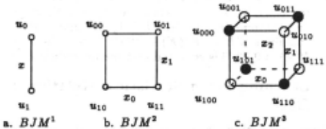
The parallel reasoning procedure in BJM is as follows:
- Before reasoning, each unit u; of the BJM is as signed a prior probability P(u;) = P< 0 >(s;).
- When we observe some evidence which creates a set of constraints {P(Sr)}, the corresponding prior {P< 0 >(S1)} is calculated by accumulation of {P(s; .. )}, and the results are distributed at each s; E Sr. For a B J Mm, if we have an n--th order constraint set, then we need m - n addition cycles to complete both accumulation and distribution.
- Each unit u; calculates its posterior P( s;) by (2) in parallel using the above results and only one multi plication cycle and one division cycle are needed to complete the computation in this step.
For the BJ M 3 in Fig. 1 c, to calculate p(O)(zo, z1) in step 2, we need add the corresponding prior of the two planes X2 : (P(uaoo), P(u1oo), P(uuo), P(ua10)) and X2 : (P(Uool), P(u1o1), P(uu1), P(uau)) to each other in parallel. 3 - 2 = 1 addition cycle is needed to complete both accumulation and distribution of the results. If we want p(O)(zo) instead of p(o)(zo, z1), then add the corresponding prior of the two planes X1 : (P(uaoo), P(Uool), P(u1o1), P(u1oo)) and X1 : (P(Uolo), P(uau), P(um), P(uuo)) to each other, and then add the corresponding results on planes X2 and X2 to each other. Here, we need 3- 1 = 2 addition cycles.
Example 1 (XOR Problem): For the exclusive-or (XOR) problem (Table 1), a 3-dimensional BJM (Fig.
| lnput | Output | MLP | ||
|---|---|---|---|---|
| zo | Z1 | Z2 | Output z2 | Error |
| 0 | 0 | 0 | 0.0095 | 0.0095 |
| 0 | 1 | 1 | 0.9913 | 0.0087 |
| 1 | 0 | 1 | 0.9913 | 0.0087 |
| 1 | 1 | 0 | 0.0109 | 0.0109 |
1c) is needed. The first step is to store the patterns to be recognized. From Table 1, we can easily obtain the conditional probabilities: P(z:~lzo, zl) = P(z:~lzo, zl) = P(z:~lzo,zl) = P(z:~lzo,zl) = 0. Thus, P(io,zl,z:~) = P(zo,zl,z:~) = P(zo,zl,z:~) = P(zo,zl,z:~) = 0. Using (1) and the above probabilities as constraints to update a flat distribution of { z0 , z 11 z:~}, we ob tain P(zo, i1, :&::~) = P(io, z1, z:~) = P(zo, :&1, z:~) = P(zo, z1, z:~) = 0.25. Thus, we store a probability 0.25 at each of 4 units Uooo, Uou, u1o11 and uuo (black node in Fig. 1c) and store probability 0.0 in each of the other 4 units. Actually, we do not even need these 4 units with 0 probabilities because it is easy to see from (2) that they will always keep the value 0 during any reasoning.
After storing the patterns, the recall is simply per formed by (2). The prior probabilities of the input P(io, i1) = 0.25, P(io, z1) = 0.25, P(zo, i1) = 0.25, P(z0 , zl) = 0.25 can be obtained in only one addition cycle. Suppose we have input zo = 0 and z1 = 0. The posterior state probabilities can be obtained by Jeffrey's updating in one division and one multiplica tion cycles. The only non-zero one among them is P(i0 , i 1, :&::~) = 0.25 · ~l~ = 1.0, and we have P(i:~) = 1 after two more addition cycles. That is, the output is z:~ = 0. It is easy to test all the other cases using (2).
In summary, we have a time efficient parallel reason ing algorithm for BJM. However, the number of units in a BJM exponentially grows as the number of variables increases although we may save all units which have zero probabilities in BJMs with sparse spaces.
One way to handle the exponential explosion of the number of units in a big BJM is to decompose the BJM into a network of small BJMs (called BJMNet). If we can keep the size of the biggest sub-BJM in the BJMNet fixed, the exponential explosion is avoided.
To keep the consistency of the reasoning results among the small BJMs, it is desirable to organize the BJMNet as an acyclic hypergraph [Beeri et a.l., July 1983]. Each BJM in the BJMNet corresponds to a hyperedge in the hypergraph and is an autonomous component which has its own prior distribution and always checks its interfaces with its neighbors which affect it. BJ M, is affected by BJ M; if BJ M, is the Running Intersection Predeces sor (RIP) or one of the Running Intersection Succes sors (RIS's, [Beeri et a.l., July 1983}) of BJ M;. If there is any belief change in the interfaces it will update its own distribution using (2), and then propagate the belief changes to its other RIP and RIS's. The new changes, in turn, may cause some other BJMs to update their distri butions. The network reaches an equilibrium when the gradients of all the original disturbing points are in some small ranges specified beforehand. The network can be reconfigured dynamically using some techniques such as microprogramming to fit it for different applications.
Based on the MCE principle and the theory of Markov fields we have proven [Wen, July 1989]
- Theorem 2.1: For an acyclic BJMNet, the following updating procedures are equivalent:
- Global updating the whole network with single marginal constraint set by (2).
- Local updating one sub-BJM which contains the constraints and Jeffrey propagation of the result to the whole BJMNet through the run ning intersections.
- Example 2 [Cooper, 1984]: Metastatic cancer (A) is a possible cause of a brain tumor (C) and is also an explanation for increased total serum calcium (B). In turn, either of these could explain a patient falling into a coma (D). Severe headache (E) is also possibly associated with a brain tumor.
The BN and BJMNet for this example are shown in Fig. 2, where the arrows in Fig. 2b show the RIP /RIS re lationship between BJMs. The BJM without decom-
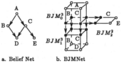
position has 5 binary variables and thus 32 units. Af ter decomposition using the techniques in [Lauritzen and Spiegelhalter, 1988; Wen, 1990b], the BJM is de composed into 3 sub-BJMs: {A, B, C}, {B, C, D}, and {C, E}. Only 2 3 + 2 3 + 2 3 = 20 units are needed here. Further saving can be achieved considering that the units in the intersections (the black nodes in Fig. 2b) are never active simultaneously (14 units are needed here).
Suppose we have an initial distribution in which It is easy to calculate the initial marginal distributions for each of the sub-BJMs:
| P(BIA) | 0.2, | P(BIA) | 0.8, |
| P(CIA) | 0.05, | P(CIA) | 0.2, |
| P(DIB,C) | 0.05, | P(DIB,C) | 0.8, |
| P(DIB,C) | 0.8, | P(DIB,C) | 0.8 |
| P(EIC) | = 0.6, | P(EIC) | 0.8, |
| P(A) | 0.2. |
| BJMg (P(A,B,C)): | 0.608, | 0.032, | 0.152, | 0.008, |
| 0.032, | 0.008, | 0.128, | 0.032. | |
| BJ Ml (P(B, C, D)) : | 0.608, | 0.032, | 0.008, | 0.032, |
| 0.056, | 0.224, | 0.008, | 0.032. | |
| BJ M? (P(C, E)): | 0.368, | 0.552, | 0.016, | 0.064. |
If we have observed P(D) = 0 and P(E) = 1, respec tively, what is the possibility that a patient suffers from metastatic cancer? The reasoning is as follows:
- BJM? uses the constraint P(E) = 1 to update its own distribution in parallel and calculates the pos terior P'(C), and broadcast it.
- Only BJM~ is affected by BJM?, and it updates its distribution with P'(C), and calculates the pos terior P'(B,C), and broadcast it.
- BJMl receives P'(B,C) from BJM~, updates its own distribution in parallel, and calculates pos terior P'(D). At this point, we finish the first step of parallel reasoning. Because the gradient V D = P'(D)- P(D) # O, the updating continues.
- BJ M~ uses another constraint P(D) = 0 to update its distribution, calculates the posterior P"(B, C), and broadcast P" ( B, C) to the network.
- BJMg and BJM~ receive P"(B,C) and P"(C), respectively, and use them to update their own distributions in parallel. BJ M? calculates P"(E) and finds V E = P"(E) - P(E) = 0. The result P(A) = 0.0973 is reported and the procedure stops.
3 Learning From Statistical Relational Data
Normally, learning starts from a sample database. Most of the contemporary databases are relational. In [Wen, 1990a], some relationships between Relational Databases (RDB) [Ullman, 1982] and BN are discovered. These in clude the correspondences bet'!een (1) functional depen dency (-+) and probabilistic dependency, a special cases of multivalued dependency ( -+-+ ), in RDB and condi tional probability in BN. (2) acyclic database scheme with join dependency in RDB and acyclic decomposition of BN. and (3) three main operations on RDB (projec tion, selection, and join) and three main operations of BN (belief extracting, updating, and propagation).
- Definition 3.1: The frequencr of an attribute subset X ofrelation schemeR in a relation ron R is Fx(R) = {Fx=z(r) = lax~j(r)l ;Vz E Dx} where Dx is the domain of X, lr I is the cardinality of r, and cr is the selection operator in RDB.
Definition 3.2: The conditional frequencr of X in r given Y = y, Y C R is
Definition 3.3: Let X, Y C R, and Z = R- XY. r satisfies the probabilutic dependencr X 1-+ Y if
According to the law of large numbers, it is rea sonable to assume liillJrl-+oo F.,(r) = P(X = z), limlrl-+oo Fx=z]Y=y{r) = P(X = ziY = y), and if X 1--+ Y then P(Y IX Z) = P(Y IX), ie. Y is conditionally independent of Z given X. It is easy to prove
Theorem 3.1 [Wen, 1990a]:
(see [Ullman, 1982] for definitions of--+ and --+--+.)
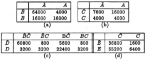
In Example 2, suppose we have the statistical informa tion in Table 2 from a sample database. Each entry of the table gives the number of occurrences of the records in the database which contain various combinations of the attributes A, B, C, D, and E. This information
| !JE | !JE | DE | DE | |
|---|---|---|---|---|
| ABC | 23104 | 34656 | 1216 | 1824 |
| ABc | 128 | 512 | 512 | 2048 |
| ABC | 1216 | 1824 | 4864 | 7296 |
| ABC | 32 | 128 | 128 | 512 |
| ABC | 1216 | 1824 | 64 | 96 |
| ABC | 32 | 128 | 128 | 512 |
| ABC | 1024 | 1536 | 4096 | 6144 |
| ABC | 128 | 512 | 512 | 2048 |
can be obtained by a projection of a universal relation of the database on {A, B, C, D, E} without eliminating the duplicates. We can easily check that the probabilis tic dependencies A 1--+ B, A 1--+ C, B, C 1--+ D, and C 1--+ E hold. According to Theorem 3.1, we can use the algorithms given in [Ullman, 1982] to decompose re lation ABCDE into 4 subrelations AB, AC, BCD, and CE with a loBBless join property. All of these relations are in 4th normal form and keep the original dependen cies projected to the corresponding relations. Thus, we can readily learn the conditional probabilities for Exam ple 2 given in section 2 from the statistical information (see Table 3) in the decomposed relations using
- The frequency method: For example, P(A) iooo+ilm$l:&:+t6000 = 0.2 and P(BIA) = 4oJ>~6000 = 0.8, etc.
- The incremental methods [Lauritzen and Spiegel halter, 1988]: suppose we have a prior P(BIA) =
| A | A | A | |
|---|---|---|---|
| B | 64000 | 4000 | 16000 |
| B | 16000 (a) | 16000 | 4000 |
| c | |
|---|---|
| 1600 | |
| D | 6400 |
~ and the next example e comes. The updated value of P(BIA) is
The above learning procedure may be trivial if the database is complete. However, we often cannot obtain a completely specified database in many practical cases. In these cases, we may have to choose one of the fol lowing methods to generalize the incomplete statistical information to a complete conditional distribution.
3.1 Floor Method And ME/MCE Method
Floor method assigns a small nonzero probability to the states (tuples) which do not occur in the database. This adds the pOBBibility of Jeffrey updating to these states. However, this method makes no distinction between the cases which are impoBBible and those which could be en countered in the future.
Similarly, ME/MCE method or Dirichlet distribution [Herskovitz and Cooper, 1990] simply assigns a uniform conditional distribution to the unseen cases. It uses for mula P(X = ziiTx = 1rx) = 0 ~n:·~:x)~:'v~ 1 to obtain a conditional distribution, where X is a variable in the underlying BN, z is one of the Vx values can be taken by X, ITx is the set of parents of X, 1r x is a particular instantiation of ITx, and C(~) is the number of tuples in the database that match the instantiated set of vari ables ~. For the unseen cases, the above conditional distribution becomes Jx and thus is uniform.
3.2 Connectionist Methods
The connectionist learning methods are interesting be cause of their generalisation ability. It has been proven that the output class probabilities of Multilayer Percep tron (MLP) and Boltzmann machine are good approx imations of the conditional probabilities needed by BN [Bourlard and Wellekens, 1990; Laskey, 1990]. In Exam ple 2, using an MLP network with 2 input units, 2 hidden units, and 1 output unit, we can learn P(DIB, C) in leBB than 100 epochs. The results are given in Fig. 4. For example, in Fig. 4a, data for P(DIB, C) are miBBing. After the network has learned the weights from the in complete data we feed B = C = 1 to the network and get an output P(DIB, C)= 0.82.
3.3 NN/OR Method
According to the Nearest Neighborhood (NN) principle, the conditional probability assigned to an unseen case for the database depends on its neighbor conditional distri butions. That is, if the unseen case has many neigh bors who have high conditional probabilities then it is assigned a relatively high conditional probability, other wise, it is assigned a low or even aero conditional prob ability. This method should be used with the Occam's Razor (OR) principle when there are two or more near est neighbors having different conditional probabilities. When there are more than one candidate hypotheses for a given problem the OR principle chooses the simplest one which is compatible or at least 90% consistent with the observed data. There are many criteria of simplic ity, eg. Kolmogorov complexity, Minimum Description Length, Formula complexity, etc. We use formula com plexity in the following examples.
Example 3: Suppose we have the training data in Fig. 3a with the functional dependency z, y, z -+ w. The
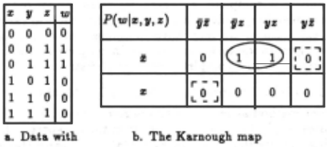
information about P( wjz, y, i) and P( wjz, y, .z) is miBBing. ME/MCE methods assign l to both of these conditional probabilities. This is obviously inconsistent with the aBBumption of z, y, z -+ w. It is easy to determine P(wjz,y,i) = 0 accord ing to the NN principle because all of its nearest neighbors have values 0 (see Fig. 3b). P(wjz,y,.Z) is more difficult to determine because its nearest neighbors have difFerent values. Considering Fig. 3b as a Karnough map, and trying to assign 0 and 1 to the entry corresponding to P(wjz,y,.z), we have two logic expreBBions zz and zz + zy, respec tively. The OR method always prefers the assign ment with the simplest expression and thus aBBigns P(wjz,y.z) = 0.
This method can be generalized to the case of proba bilistic dependencies. In Example 2, suppose the sta tistical information about P(DjB, C) (the last column in Table 3c) is miBBing. According to the NN princi ple, it is easy to determine P(DjB, C) = 0.8 {Fig. 4a). However, if the information about P{DIB, C) is miBBing latter (0.05 x iJC + 0.8 x (B +C)), we prefer the first choice (see Fig. 4b). Similarly, we have the conditional probabilities learned for P(DjBC) and P(DjiJC) when the corresponding information miBBing (Fig. 4c,d).
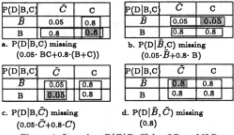
{Fig. 4b), we may have two choices for it: 0.05 and 0.8. Because the former has a probabilistic logic expreBBion 0.05 x B + 0.8 x B which is simpler than that of the
4 Performance and Comparisons
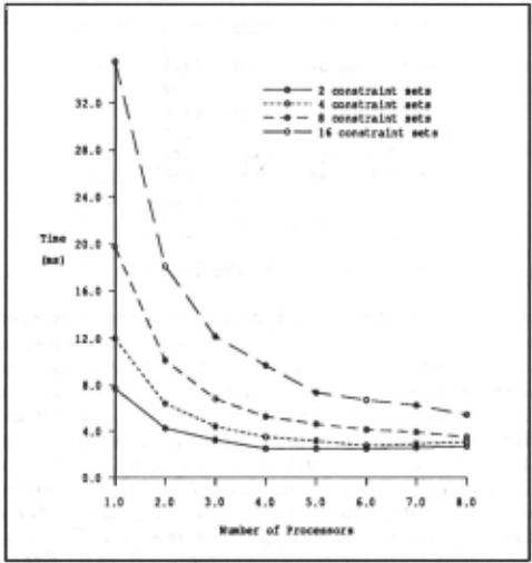
A number of typical examples of reasoning have been tested to evaluate the performance of the BJM model. Fig. 4 gives the results of one of our experiments, which uses a 10-dimensional BJM. Fig. 4 shows the results for the reasoning cases with 2,4,8,16 constraints and 1-8 par allel simulated proceBBing units {threads for the Encore Computer). It is easy to see that the speed up is quite satisfactory when the ratio No.unit· is small For No.Coo;vtrc&·f.lt· · greater ratio, the performance suners trom the parallel scheduling overhead a bit.
Comparing with perceptron models, our model has its obvious advantages. [Minsky and Papert, 1969] showed that no single-layer perceptron can solve XOR problem. For CES/MLP, using backpropagation method [Rumel hart et al., 1986], a total sum of squares (tBB) 0.0398 is obtained after 298 epochs of training in a feedforward network with 2 input units, 2 hidden units, and 1 out put unit. The test result for all the patterns is given in Table 1. From this example, it can be seen that for recall from completely specified distributions of sparse spaces, the BJM model outperforms CES/MLP model in the following aspects: ( 1) No time-consuming learning procedure is involved. {2) Only addition, multiplication, and division operations but not complicated calculations like sigmoid are needed. {3) The result is accurate. (4) The reasoning direction can be arbitrary. {5) The net work structure is much more regular than CES/MLP. The granularity of BJMNet is also good.
For large scale applications, neither MLP nor BJM are Probablr. Approximately Correctly (PAC) learnable [Judd, 1987 . However, in [Wen, 1990a] we have proven
- Theorem 4.1: If the maximum BJM in the BJMNet has a fixed size, the BJMNet is PAC learnable from statistical relational data.
It is possible to decompose an MLP network in a way similar to that of BJMNet. Gallant's connectionist ex pert systems [Gallant, Feb 1988] may be thought of as one step towards this direction. However, Gallant's method can handle only functional dependencies but not probabilistic dependencies, and does not work properly for problems like Example 2.
5 Conclusions
A parallel distributed model for reasoning/learning is proposed based on BN paradigm. Issues about the struc ture, learning methods, and the reasoning method for the model are discussed. Comparison between BJMNet and CES shows that the soundness and efficiency of the model can be guaranteed for a wide range of applica tions:
- The model has probability theory and information theory as its theoretical basis.
- It can be implemented automatically by a set of learning methods from statistical relational data.
- Reasoning in this model can be in any directions, in contrast to the CES models which can only reason in single direction [Gallant, Feb 1988].
- NP-hardness in both reasoning and learning is handled by decomposing the BN into small BJMs.
A prototype of simulator of BJMNet has been developed for the Encore Computer, a shared memory multiproces sor system [Wen, Nov 1989].
Acknowledgement
Thanks to E. A. Sonenberg, B. Marksjo, A. Kowalczyk, H. Liu, and L. Fang for discussions and comments. The permission of the Executive General Manager, TRL, to publish this paper is gratefully acknowledged.
@inproceedings{ijcai1991p178,
  title     = {Parallel Distributed Belief Networks That Learn},
  author    = {Wen, Wilson X. and Jennings, Andrew},
  booktitle = {Proceedings of the Twelfth International Joint Conference on
               Artificial Intelligence, {IJCAI-91}},
  publisher = {International Joint Conferences on Artificial Intelligence},
  editor    = {John Mylopoulos and Ray Reiter},
  pages     = {1210--1217},
  year      = {1991},
  month     = {8},
  note      = {Qualitative Reasoning},
  url       = {https://ijcai.org/proceedings/1991/178},
}
TY - CPAPER TI - Parallel Distributed Belief Networks That Learn AU - Wen, Wilson X. AU - Jennings, Andrew T2 - Proceedings of the Twelfth International Joint Conference on Artificial Intelligence, IJCAI-91 PB - International Joint Conferences on Artificial Intelligence PY - 1991 SP - 1210 EP - 1217 UR - https://ijcai.org/proceedings/1991/178 ER -Copied
Machine-readable versions of this paper, for tools and AI agents:





