
Combining Qualitative and Quantitative Knowledge to Generate Models of Physical Systems
Proceedings of the Twelfth International Joint Conference on Artificial Intelligence. Qualitative Reasoning. Pages 1158-1162.
© 1991 International Joint Conferences on Artificial Intelligence
Abstract
All major approaches to Qualitative Reasoning rely on the existence of a model of the physical system. However, the task of finding a model is usually far from trivial. Within the area of electrical engineering, model building methods have been developed to automatically deduce models from measurements . In this paper we explicitly show how to incorporate qualitative knowledge in order to apply these methods to situations where they do not behave satisfactorily. A program has been developed and applied to a non-trivial example. The qualitative input, in terms of an incomplete bond graph, and the resulting output can be used to form a more complete bond graph. This more informative model is suitable for further reasoning.
- [Andersson, 1985] Peter Andersson. Adaptive forgetting in recursive identification through multiple models. Int. Journal of Control, 42(5):1175-1193, 1985.
- [Breiman et a/., 1984] L. Breiman, J .H. Friedman, R.A . Olshen, and C.J . Stone. Classification and regression trees. Wadsworth & Brooks, Monterey, 1984.
- [Forbus and Falkenhainer, 1990] K.D. Forbus and B. Falkenhainer. Self-explanatory simu- lations: An integration of qualitative and quantita- tive knowledge. In Proc . of the Eighth National Conf. on Artificial Intelligence (AAAI-90} , pages 380-388, 1990.
- [Gustafsson and Stromberg, 1989] F. Gustafsson and J .E. Stromberg. Estimating model trees for describ- ing piecewise linear systems. Technical Report LiTH- ISY-1-1030, Dept. of Electrical Engineering, Link oping University, Sweden, 1989.
- [Gustafsson, 1990] Fredrik Gustafsson. Optimal seg- mentation of linear regression parameters. LIU- TEK-LIC-1990 :46, Dept. of Electrical Engineering, Linkoping University, Sweden, 1990.
- [Karnopp and Rosenberg, 1983] D.C. Karnopp and R. Rosenberg. Introduction to physical system dynamics. McGraw-Hill, New York, 1983.
- [Kuipers and Berleant, 1988] B. Kuipers and D. Berleant. Using quantitative knowledge in qual- itative reasoning. In Proc. of Seventh National Conf. on Artificial Intelligence ( AAAI-88}, 1988.
- [Kuipers, 1986] Benjamin Kuipers . Qualitative simula- tion. Artificial Intelligence, 29:289-338, 1986.
- [Ljung, 1987] Lennart Ljung. System identification - Theory for the user. Prentice-Hall, Englewood Cliffs, New Jersey, 1987.
- [Top and Akkermans, 1990] J .1. Top and H. Akker- mans. Bond graph based reasoning about physical systems. In Proc. Workshop on Model-Based Reason- ing (AAAI-90}, 1990.
- [Top et a/., 1991] J .L. Top, J .M . Akkermans, and P.C. Breedveld. Qualitative reasoning about physical sys- tems: an artificial intelligence perspective. Journal of The Franklin Institute, April(To appear), 1991. Spe- cial bond graph issue.
References were extracted automatically from the PDF and may contain errors.
Full text extracted automatically from the PDF; figures, tables and equations may differ. The PDF is the version of record.
1 Introduction
The major approaches to qualitative reasoning (QR), all rely on the existence of a model of the physical system. All of them have developed model languages, that is, languages for representing qualitative knowledge about physical systems, as well as methods for reasoning qual itatively within these languages. However, since real systems, both man-made and natural, are often com plicated, the task of finding a model is usually far from trivial.
Much work in the area of model building has tradition ally been performed by engineers with the goal of build ing controllers for industrial systems and for building simulators. In this case, the goal is to find quantitative models, usually in terms of differential equations, such that they mimic the input/output behavior of the phys ical system. To automize the model building process, methods have been developed to deduce models from measurements. This art of fitting a sufficiently complex model structure to a given set of measurements, is re ferred to as system identification.
In this paper, we will consider a class of physical sys tems for which conventional system identification does not behave satisfactorily. For this class we show how to introduce qualitative knowledge to support the sys tem identification. A program has been developed and applied to a non-trivial example. The qualitative in- Jan-Erik Stromberg Dept. of Electrical Engineering, Linkoping University S-581 83 Linkoping, Sweden Email: janerik@isy.liu.se
put, in terms of an incomplete bond graph, and the resulting output can be used to form a more complete bond graph [Karnopp and Rosenberg, 1983]. An incom plete bond graph is, in our context, a graph without constitutive relations - compare e.g. an electrical cir cuit where the component values are unknown. This completed bond graph is more informative and is suit able for further reasoning [Top and Akkermans, 1990, Top et a/., 1991].
Hence, we will assume the following three types of knowledge are at hand: general knowledge of physics and physical systems, specific (possibly partial) knowledge of the system considered and empirical data in terms of measurements from the system. Since the measured data is assumed to come from a real system, it may also con tain noise. Finally, the illustrating example will be taken from the class of piecewise linear systems, i.e. systems with discrete non-linearities only.
Some other researchers have also worked in the area of integrating quantitative and qualitative knowledge. Kuipers and Berleant [1988] use quantitative knowledge to refine predictions of a qualitative reasoner which rely on an already existing model. However, they do not address the model building problem itself. Forbus and Falkenhainer [1990], on the other hand, work with model building. They use a qualitative model to produce an en visionment for the physical system. The envisionment is then used together with a mathematical model library to build quantitative models. This requires exact knowl edge about the mathematical models that describe the system parts. Our approach to model building differs in that we do not require any such knowledge. We use the measured data to derive the corresponding information.
The section to follow gives a brief introduction to con ventional system identification. In Section 3, we intro duce our model structure proposal - a bond graph based approach. Section 4 explicitly describes how to incorpo rate the qualitative knowledge from the model in Section 3. Section 5 gives a short conclusion of our results.
2 Conventional system identification
System identification (SI) is the art of fitting a chosen model structure to a set of measurements given from a physical process. If the model structure is chosen among the set of linear differential equations, there is a rich flora of general methods as well as a good understanding for how they behave (see [Ljung, 1987] for an overview). As a matter of fact, these methods behave well, in the sense that they produce models good at imitating the in put/output behavior of the physical system, even if the system is not perfectly linear. However we do require the non-linearities to be fairly "small". When this assump tion no longer holds true, the flora of general methods shrinks quickly.
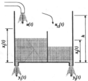
In this section we consider one fairly general method called AFMM (Adaptive Forgetting through Multiple Models) [Andersson, 1985] suitable for piecewise linear systems, Le. systems abruptly changing between linear modes of operation.
The example and its model structure: As an il lustrating example consider the water tank with a sep arating wall as depicted in Figure 1. For simplicity, as sume a linear relationship between water levels and out flow. This system is piecewise linear with its discrete non-linearities appearing when the water levels reach the edge of the separating wall. Using some basic insight into physical systems modeling, we will find the following set of differential equations (a state-space model) being a suitable structure for the tank:
The state variables x1 (t) and x2(t) represent the water levels in the left and right halves respectively. Here we have used the convention x(t) = da\t). The aii :s and bi :s are the unknown parameters we want to identify. However, we notice that the values of these parameters will undergo abrupt changes as the water levels vary in time. These changes naturally correspond to the water levels passing the edge of the wall.
2.1 AFMM: Segmenting abruptly changing systems
SI algorithms may in fact be considered as time vary ing filters. These filters take the measurements as input and generate as output estimates of the unknown pa rameters of the underlying equation. The key idea of AFMM is to set up M such filters in parallel (multiple models). All these will normally work independently of each other and if initialized appropriately, some filters will produce better estimates than the other at a given time instant. It can be shown that an optimal filter for solving a linear SI problem will have a "time constant" that increases monotonically in time. This means that the best estimator will also be the slowest to adapt to changes. Therefore, by keep resetting the time constants of (some of) the filters performing badly, we enable the filter most recently reset to respond to an abrupt change in dynamics. This latter strategy is the adaptive forget ting part of AFMM.
Given measurements and a model structure in terms of linear differential equations, AFMM will produce esti mates of the jump-times as well as parameter estimates for each time segment between detected jumps. Opti mality aspects of this and related strategies are thor oughly discussed in [Gustafsson, 1990] .
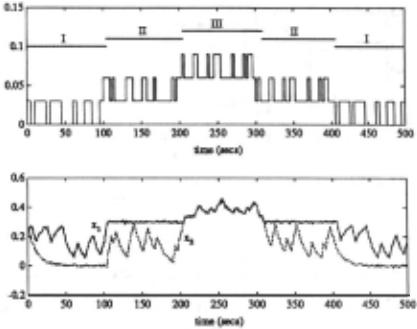
AFMM applied to the example: In Figure 2 we plot the sampled measurements of a simulated version of the water tank. In order to mimic the noise present for real measurements, we have added a sequence of in dependent random variables, i.e. white noise, to the simulated output levels. It can be shown that the be havior of the tank may be separated into three distinct modes of operation. For each such mode, all the a- and b-parameters of (1) are time invariant constants. The horizontal line segments in the upper diagram represent these modes (roman numbers).
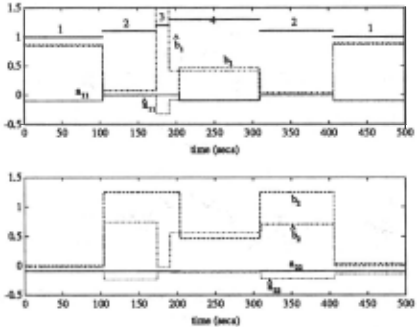
In this simulation, the height h of the separating wall is taken to be 0.3 units and the sampling time is assumed to be 1 second. The input flow u(t) is chosen as to force the system into all of its operating modes. The noisy versions of x1(t), x2(t) and the noise free input flow u(t) are taken as input to AFMM. The resulting parameter estimates (together with the "true" parameter values) are depicted in Figure 3. We notice the following:
- The time instants at which the real jumps occur are reasonably well estimated. However, there is also a "faulty" jump detection. This is quite a common problem with this kind of sub-optimal segmenta tion strategy. False jump detections are due to the method being unable to separate noise from true mode switching. In order to handle this problem
of noise separation, AFMM critically depends on a noise variance estimate. Unfortunately this estima tion problem is known to be hard in its own.
- Not only is the estimation error quite large, but also are the estimates varying inside the same mode of operation. How do we conclude that the b2 esti mates in the second and fifth time segments actually correspond to the same operating mode?
2.2 XAFMM: Clustering the segmentation
As a by-product from the filters used in AFMM, we also get estimates of the variance of the parameter estimates. This enable us to formulate a statistical test to check whether estimates from two different segments are likely to correspond to the same operating mode, i.e. the same dynamical description. This test has been implemented in an extended version of AFMM (XAFMM) and could solve the second problem observed in the previous sub section. The output from XAFMM consists of two parts: the lumped parameter estimates and corresponding seg ment labels.
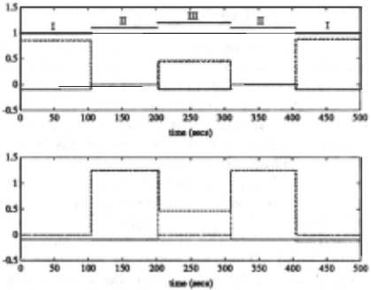
XAFMM applied to the example: The segment la bel output from XAFMM is depicted as horizontal line segments at the top of Figure 3. The labels generated have no other meaning than telling which parameter esti mates have been lumped together by the statistical tests. Hence, they do not necessarily correspond to the operat ing mode labels of the upper diagram in Figure 2. How ever, without any further knowledge, we have to accept these labels as reflecting our current notion of the "op erating mode" . We also notice the following:
- Given the chosen strength of the statistical tests, XAFMM did not manage to remove the "faulty" jump detection. Hence, knowing nothing else about the physical system, we have to conclude the system has four different modes of operation.
- Since we have been able to label the lumped esti mates, we may now take this as input to a statisti-
cal classifier to form an immediate mapping from a measurement sample to the corresponding operat ing mode.
2.3 Building model trees
Regression trees are binary tree structured classifiers where the internal nodes correspond to tests on some feature vector and the leaves are the class labels . In [Breiman et al., 1984] we find a statistically based method for inferring regression trees from measurements once they have been class labeled. This is obviously a suitable tool for finding the mapping from a measure ment sample to the corresponding operating mode of the process. When using regression trees to describe this particular mapping, i.e. when the class labels cor respond to operating modes, we call this construction a model tree.
Using the estimated operating modes from XAFMM, we notice that the state variables (in the example x1 and x 2 ) should be taken as elements in the feature vector and the labels produced by the clustering procedure as "class labels" . Details about the implementation of XAFMM and the related tree growing procedure, may be found in [Gustafsson and Stromberg, 1989].
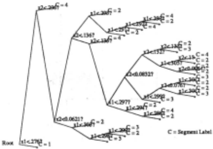
Tree building applied to the example: Using the segment labels produced by XAFMM as depicted in Fig ure 3, we end up in the tree in Figure 4. We have used simple threshold type of node questions "x; < r?", but other questions could be used. We notice that it is dif ficult to interpret the obtained tree. The main reasons for this being the case, are:
- We have an incompatible number of operating modes due to the "faulty" jump detection. Since this jump has no relevance in the physical system, the tree builder will have a difficult task in trying to ~xplain this jump in terms of the "real" state variables.
- Not even the real jump-times are perfectly esti mated. This also seriously affects the possibility to find the relevant questions.
3 The modeling language
To master the problems observed above, we will take the approach to use qualitative knowledge. We will represent the qualitative knowledge in terms of an incomplete bond graph. A bond graph represents energy processes in a physical system. It has a small number of primitive en ergy processing elements: source, storage, dissipator and transformer. These elements are connected in a graph via energy bonds (drawn as half arrows) and two spe cial junctions. For each bond there are two generalized power variables called effort and flow. Their product is power and represents the energy flowing through that particular bond. The two junctions represent connec tions where one of the two power variables is common to all connected bonds. For example, parallel and serial connections in electrical circuits are connections where the power variables voltage and current respectively are common to the connected components. A common effort junction is represented by a "0" and a common flow by a "1".
The time integrals of the power variables flow and effort are called displacement and momentum, respec tively. These are usually referred to as energy variables. The functioning of each energy-processing element is ex pressed in terms of a constitutive relation between two variables. Energy dissipators relate two power variables and storage elements relate one power and one energy variable. An electrical resistor is a dissipator and its constitutive relation known as Ohm's law. A water tank is a fluid storage where the tank properties are reflected in a constitutive relation between pressure (effort) and amount of water (displacement, if water :Bow is defined as the abstract :Bow variable). Defining constitutive re lations this way, they always become static.
3.1 A bond graph representation of the example
The bond graph for the tank is shown in Figure 5. There are four junctions in the graph. The 0-junctions repre sent the pressures, or equivalently the water levels, in each half of the tank. The !-junctions represent the wa ter flow between the two halves. The left and right 0junctions are for the left and right halves of the tank, respectively. The 1-junction in . between the 0-junctions represents an abstract water flow from left to right when the two water levels are strictly above the edge of the wall, i.e. the tank will behave as if the wall did not exist at all. The 1-junction to the left represents the physical flow appearing when the left water level reaches the edge of the wall while the right level is below (or possibly at) the edge. For a water level below the edge, the flow be tween the halves is always zero and the two halves are completely disconnected.
The energy processing elements C1 , C2 represent the two separate halves of the tank. R1 , R2 represent the outflow characteristics of the holes 'in the bottom of the two halves. SJ represents the source generating the in flow to the tank system- from a black-box point of view, this is our exogenous input signal u(t). The abstract source sh~ is introduced to model the physical flow from left to right half of the tank. The amount of flow generated by sh~ is defined to be equal to Q~2 via a active bond (full arrow) originated at the left 1-junction. The remaining elements are used to control the mode switch ing of the system. The two modulated R-elements M R1 and M R2 can be thought of as "valves" connecting the left and right halves by closing and opening appropri ately. M R1 is used to control the flow in order to make the levels equal when the water levels are strictly above the edge of the wall. M R2 is used to control the flow in order to make the left level :=:; h while the right level is below (or at) the edge.
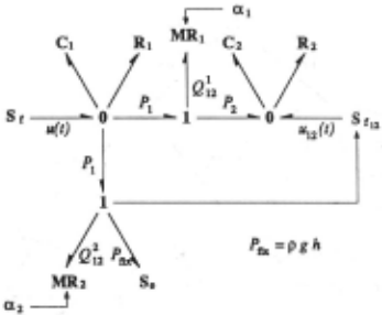
To control the two modulated elements we use two sig nals a1 and a2 being discrete binary signals determining the flow resistance of the "valves". The signals take the values infinite (closed valve) or zero (open valve). When the water levels are strictly above the edge of the wall, a1 is zero (valve M R1 opened) and a2 is infinite (valve M R2 closed). In this case, a pressure difference P1 - P2 over the valve M R1 will always be neutralized via an appropriate flow Ql 2 · Since M R2 is closed, Q~2 will be identical to zero even if the pressure difference P1 - PJi:r: is varying. When the left level is at the edge and the right level is below (or at) the edge, M R2 is opened and M R1 closed. If the water pressure P1 differs from the fixed pressure PJi:r: given by the pressure source s., we get a nonzero flow Q~2 · This is exactly the outflow from the left half necessary to keep the left level :::; h. There fore the same flow should enter the right half, which is taken care of by the flow source Sh~. When both the water levels are below the edge, both valves are closed.
Obviously, the signals a 1 and a 2 are functions of the water levels in the following manner:
This will be referred to as the discrete control field of the bond graph.
3.2 The model tree representation
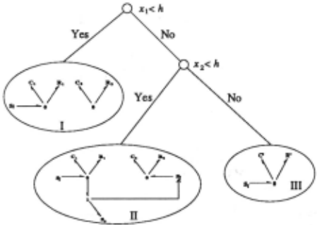
The signal combinations define regions in the state space. In each of these regions the system is described by different linear region models. The qualitative description of each region model can be inferred from the bond graph by setting up all the different combinations (a limited number) of signals and for each such combination, sim plify the bond graph. In our example, this process results in three simplified bond graphs which, together with the control field (2), form another qualitative description. This alternative model structure is a model tree. In this particular case, the leaves are simplified bond graphs and the conditions at the internal nodes are the binary ques tions asked in the control field (2) . The working example is represented by the model tree in Figure 6.
4 Incorporating qualitative information
Now we will look at some specific ways in which the qualitative information according to Section 3, can be incorporated in order to master the problems.
4.1 IAFMM: Interpreting the segmentation
In order to incorporate any of the qualitative information given in terms of a correct but not necessarily complete bond graph, we need to interpret the results generated by XAFMM in terms of this data structure. This however is a problem. Take for instance the labels generated by the clustering routine of XAFMM. Even the total number of labels are incompatible with the number of leaves in Figure 6. Therefore, we must first introduce some means of connecting the operating mode labels of Figure 6 with the labels produced by XAFMM.
As outlined in Section 2.2, for each increment in time, some of the badly behaving filters are reset. When doing this, we also need tore-initialize the filters' parameter as well as variance estimates. Obviously this is an excellent opportunity to test hypothesis inspired by the informa tion contained in the bond graph. This is exactly what is done in the interpretable version of XAFMM (IAFMM) .
Basically, what we do is to take the model tree gener ated from the bond graph. We then compare the simpli fied bond graphs at the leaves with the model structure according to (1). This usually enable us to fix some of the parameters. Typical fixed values are 0 and ±1. Another common result of the bond graph reduction is that the model order can change.
Having initialized a filter according to the fixed param eter values, we finally mark the specific filter in order to keep track of the outcome of our hypothesis test. Ob viously a suitable label is the operating mode labels of Figure 6.
| Parameter: | au | a12 | bl | a21 | a22 | b2 |
|---|---|---|---|---|---|---|
| Mode 1 | "! | u | ·r | ·r | 0 | u |
| Mode II | 0 | 0 | 0 | ? | ? | ? |
| Mode III | ? | 0 | ? | - | - | - |
When initializing the estimates in AFMM we substi tute the "?" entries of the table with zeros . . The only difference between a "?" entry and a "real" 0, lies in the variance estimate initialization. If we believe in a value holding true, we set the corresponding variance es timate, i.e. the uncertainty, to some small number. The "-"-entries appearing in the Mode III-row correspond to the model reduction; the two dimensional state vector collapses into a scalar, i.e. the tank behaves as if the separating wall did not exist. The results produced by IAFMM are depicted in Figure 7. We notice the follow ing:
- The estimated parameter values are now much closer to the "true" parameter values. In fact, most of the time they do coincide.
- The estimated values are less varying within one and the same operating mode. More important however, we notice that the estimated number of modes now is correct - no faulty jump detections. The sensi tivity of AFMM on the noise variance estimate, has been relaxed.
- The jump-time estimates are slightly improved.
- The labels assigned to the segments now relate di rectly to the mode labels of Figure 6.
4.2 Improving the model tree
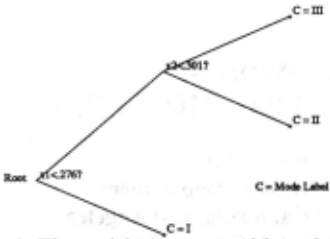
Since the tree structure is already known (Figure 6), we may now simplify the general tree building algorithm used in section 2.3. This simplified tree builder, referred to as a tree adjuster, take as input the a-priori given tree structure, and return as output the optimal node questions and leaf labels. '
Tree adjusting applied to the example: Entering the tree s~ructure given in Section 3, the tree adjuster produces the tree according to Figure 8. We notice the following:
- The labels at the leaves now relate directly to the leaves of Figure 6. This follows from the special labeling of the filters in IAFMM.
- We may now immediately interpret the resulting node questions in terms of physical parameters. In particular, the thresholds obtained obviously corre spond to the height of the separating wall .
- We may also notice a difference between the two chosen thresholds, representing a "safety margin" introduced by the measurement noise. In fact, this is exactly the kind of robustifying thresholds we would prefer, when using the tree in real applica tions (e.g. for guiding the mode switching of a con troller) .
5 Conclusion
In this paper we have suggested a method to generate models for a class of non-linear physical systems. We have shown what kind of qualitative information that may be useful in order to improve on the results of ex isting SI methods. We have also made explicit how this information may be included in a particular SI method named AFMM - a method for segmenting piecewise lin ear systems.
We have introduced the use of multi-domain bond graphs for structuring the qualitative information avail able. Also, the resulting information obtained from mea surements may be fed back to the bond graph to make it more complete. This more informative model is a good prerequisitive for further reasoning. We recognize the following two immediate possibilities:
- Extract the information needed to produce, for example qualitative constraint equations [Kuipers, 1986]. This may then be used as input to QSIM.
- Perform the reasoning directly in the bond graph. This approach has been discussed in [Top and Akkermans, 1990, Top et a/., 1991] .
@inproceedings{ijcai1991p170,
  title     = {Combining Qualitative and Quantitative Knowledge to Generate Models of Physical Systems},
  author    = {Söderman, Ulf and Strömberg, Jan-Erik},
  booktitle = {Proceedings of the Twelfth International Joint Conference on
               Artificial Intelligence, {IJCAI-91}},
  publisher = {International Joint Conferences on Artificial Intelligence},
  editor    = {John Mylopoulos and Ray Reiter},
  pages     = {1158--1162},
  year      = {1991},
  month     = {8},
  note      = {Qualitative Reasoning},
  url       = {https://ijcai.org/proceedings/1991/170},
}
TY - CPAPER TI - Combining Qualitative and Quantitative Knowledge to Generate Models of Physical Systems AU - Söderman, Ulf AU - Strömberg, Jan-Erik T2 - Proceedings of the Twelfth International Joint Conference on Artificial Intelligence, IJCAI-91 PB - International Joint Conferences on Artificial Intelligence PY - 1991 SP - 1158 EP - 1162 UR - https://ijcai.org/proceedings/1991/170 ER -Copied
Machine-readable versions of this paper, for tools and AI agents:





