Extracting and Representing Qualitative Behaviors of Complex Systems in Phase Spaces

1 Introduction

Analysis of dynamical systems via phase space structures plays an increasingly important role in experimenting, interpreting, and controlling complex systems [Abelson and Sussman, 1989a; Abelson et a/., 1989b]. Nonlin­ ear systems usually fall outside the domain of tradi­ tional analysis, such as Fourier analysis for linear sys­ tems. However , most of the important qualitative be­ haviors of a nonlinear system can be made explicit in the phase space with a phase space analysis.

*This paper describes research done at the Artificial In­ telligence Laboratory of the Massachusetts Institute of Tech­ nology, supported in part by the Advanced Research Projects Agency of the Department of Defense under Office of Naval Research contract N00014-89-J-3202, and in part by the N a­ tiona! Science Foundation grant MIP-9001651. The author is also supported by a G.Y. Chu Fellowship.

We have constructed a program, MAPS 1 , for under­ standing and representing qualitative structures of phase spaces through a combination of numerical, combinato­ rial, and geometric computations and techniques of spa­ tial reasoning. MAPS uses theoretical knowledge about nonlinear dynamical systems. We will illustrate our tech­ niques of extracting and representing the qualitative fea­ tures of the phase space structures with two and three dimensional systems. The techniques presented in this paper also apply to higher "dimensional systems.

Complex systems are often nonlinear and high dimen­ sional. Our theoretical knowledge about nonlinear dy­ namical systems is far from complete. Therefore, many engineering applications reply on extensive numerical ex­ periments. A numerical simulation typically generates an immense amount of quantitative information about a complex system. To interpret the numerical result and to use the information for engineering designs, it is essen­ tial to develop qualitative methods that automatically analyze the system, extract the qualitative features, and represent them in a high level description sensible to hu­ man beings and manipulable by other programs.

This paper demonstrates a qualitative method for automatically understanding and representing the "shapes" of dynamical systems. Our ultimate goal is to develop a class of intelligent and autonomous controllers that understand the phase spaces of complex systems, sense the world, synthesize control commands, and af­ fect the processes. For example, an intelligent controller would balance an inverted pendulum that is mounted on a moving cart pulled by a motor, through qualitatively analyzing the pendulum system, monitoring the motion of the system, and commanding the motor, much like what one would do to balance a broom on its end with a hand. Accomplishing such difficult tasks by autonomous robots would be hard to imagine without their under­ standing of the qualitative behaviors of the systems, es­ pecially when the systems are of high order and operate in nonlinear regimes. We are particularly interested in automating the control analysis and synthesis for a class of nonlinear systems that do not lend themselves easily to traditional analysis and design techniques .

1 MAPS stands for Modeler and Analyzer for Phase Spaces. See [Zhao, 1991a] for more detailed discussions on the program.

2 Automated Qualitative Analysis of Phase Space Structures

The phase spaces of nonlinear dynamical systems often consist of qualitatively different regions. The "shapes" of dynamical systems refer to the geometric information about the structures and spatial arrangements of these regions. A key component of the qualitative analysis of the "shapes" is to determine the stability regions of the dynamical system. The geometric information about the stability regions is extremely useful in analyzing sta­ bilities of control designs for complex systems, such as electric power systems and mechanical control systems, as well as in economics, ecology, etc.

MAPS understands qualitatively different regions and extracts and represents geometric shape information about these regions. Given a dynamical system specified as a system of governing equations, MAPS generates a complete, high level symbolic description of the phase space structure as the result of the analysis. The high level description can be used as input to other programs for further computations.

2.1 The qualitative phase space structures

We are interested in representing the qualitative features of dynamical systems for engineering analysis and de­ sign. For this purpose, the qualitative phase space struc­ ture of a dynamical system within the phase space region of interest is characterized by the equilibrium points and limit cycles and their stability types, the geometric struc­ tures of stability regions associated with the attractors, and the spatial arrangement of the equilibrium points, limit cycles, and stability regions.

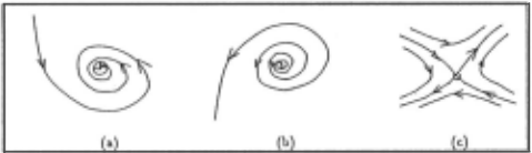
We review some of the basic concepts in dynamical system theory in order to describe the qualitative phase space structures. The equilibrium points of a dynam­ ical system x' = f(x, u), where u is a parameter, are the zeros of the vector field f( x, u) : Rn - Rn. Struc­ turally stable systems [Guckenheimer and Holmes, 1983] can have equilibrium points of three types: stable equi­ librium points ( attractors), unstable equilibrium points ( repellors), and nons table equilibrium points (saddles), whose local behaviors in phase spaces are shown in Fig­ ure 1. An attractor is an equilibrium point that nearby trajectories approach in forward time. A repellor is the one that repels nearby trajectories and can be thought of as an attractor in reverse time. Trajectories approach a saddle in some directions and leave it in the other di­ rections . . For example, the downward resting state of a damped pendulum is an attractor and the upward state is a saddle. The equilibrium points are asymp­ totic behaviors of dynamical systems. The other classes of asymptotic behaviors are limit cycles, quasi-periodic orbits, and chaotic attractors. Although our techniques apply to limit cycles and quasi-periodic orbits, we shall not discuss them in detail in this paper.

The collection of trajectories approaching an equilib­ rium point is called the stable trajectories of the point; and the collection of trajectories leaving an equilibrium point is called the unstable trajectories of the point. A saddle has stable trajectories along some directions and unstable trajectories along the other directions. The union of the stable trajectories of an attractor is its sta­ bility region, often called the basin of attraction. The important concept of stability is associated with the sta­ bility regions. The stability region of an attractor is a simply connected and open region, either bounded or un­ bounded. Every trajectory starting in the region will be attracted to the at tractor, by definition. The boundary of the region contains saddles or repellors only. The re­ gion is unbounded if the boundary contains no repellors.

2.2 Automated qualitative analysis

Our algorithm for determining stability boundaries is based on a crucial theoretical result characterizing the stability boundaries of a fairly large class of dynamical systems. Under certain weak conditions the result of Chiang et al. [Chiang et al., 1988] shows that the sta­ bility boundary for an attractor consists of the stable trajectories of equilibrium points and limit cycles whose unstable trajectories approach the at tractor. This allows us to numerically determine a collection of trajectory points on the stability boundary through calculations of the stable and unstable trajectories.

We need to extract the geometric information about the stability regions from the numerical results about the stability boundaries, and represent it parsimoniously so as to facilitate further computations. For example, the representation is to be used to estimate the volumes of the stability regions, to reason about the spatial relations with the stability boundaries, to compute topological properties of the regions, to extract information about trajectory flows, etc. Given a set of trajectory points on the stability boundary, the minimal representation­ the one with fewest edges and preserving topological structures-is the polyhedron having those boundary points as vertices. Furthermore, the polyhedron is con­ tained in the convex hull of the boundary points.

The geometric information about a stability region is represented as a polyhedron, tightly stretched over the trajectory points on the stability boundary. Extraction of the polyhedral approximation proceeds in two steps: computing a triangulation of the convex hull containing the polyhedron, and eliminating exterior triangles. The convex hull is computed and tessellated with simplices (triangles, tetrahedra, etc.) by a triangulation method­ the Delaunay triangulation. The polyhedral approxi­ mation is then extracted by a "sculpture method" used in visual information representation [Boissonnat, 1984]. Simplices exterior to the polyhedron are eliminated by heuristic rules.

2.3 The algorithm

We present the following algorithm for analyzing, ex­ tracting, and representing qualitative features of a dy­ namical system of any order in the phase space.

(1) Identify qualitative behaviors:

• (a) locate equilibrium points/limit cycles and classify their stability types;
• (b) compute stable and unstable trajectories for each saddle/limit cycle;
• (c) identify those saddles/limit cycles whose unstable trajectories approach an attractor;
• (d) the stability boundary for the at tractor is the union of the stable trajectories of those sad­ dles/limit cycles identified in (c);
• (e) check if consistency rules are violated. If yes, look for missing equilibrium points/limit cycles and go to step (a). Otherwise, go to the next step.
• Extract geometric structures:
• (a) for each attractor, collect stability boundary points;
• (b) tessellate the convex hull of the boundary points with a triangulation;
• (c) extract a polyhedral approximation to the stability region.
• Summarize qualitative behaviors:
• (a) compile the phase space data structure from step 1 into a relational graph;
• (b) augment the graph with the geometric structure from step 2;
• (c) report the graph as the output.

The set of consistency rules specify the conditions for the stability boundaries and are used in the algorithm to automatically locate missing saddles.

1. The Existence Rule: Every stability region of an at­ tractor has a boundary in a phase space with mul­ tiple attractors;
2. The Separation Rule: Separatrices either form a closed surface or become unbounded on all ends.

The first rule states the existence of stability bound­ aries in a phase space with multiple attractors. The sec­ ond rule describes the separation property of multiple stability regions. The separatrices are stability bound­ aries that separate two stability regions.

The first step of our algorithm is based on a numerical method proposed by Parker and Chua [Parker and Chua, 1989] for numerically determining stability boundaries of planar systems. We have augmented their method with the set of consistency rules they suggested to auto­ mate the locating of saddles. Since the Newton-Raphson method used in finding equilibrium points requires an initial guess, Parker-Chua's method uses a grid to set up initial guesses and is able to find all the stable and un­ stable equilibrium points under normal circumstances. However, they require that the initial guesses for saddles be provided manually by the user. We seek to automate saddle locating by focusing the search for missing saddles on the most likely places using partial boundary informa­ tion already obtained, or by refining the initial guesses for the Newton-Raphson method. We want to empha­ size that our algorithm is valid for higher dimensional systems as well and generates a symbolic description of the phase space structure. Parker-Chua's method is de­ signed for numerically analyzing planar systems only.

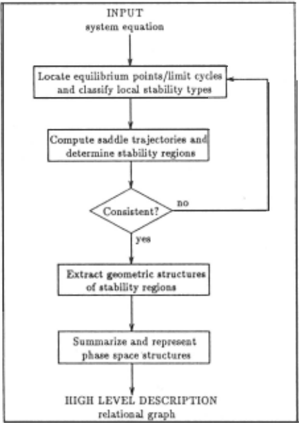
MAPS uses our algorithm to analyze the qualitative behaviors of nonlinear dynamical systems. It is imple­ mented in Scheme, a dialect of LISP. All the numerical routines are implemented in Scheme as well. Figure 2 shows the flow chart of MAPS. The input to MAPS is a system of governing equations for a dynamical system.

2.4 The main illustration

We illustrate how MAPS is used to compute the high level description of a dynamical system with an example. Consider a 2nd order nonlinear system

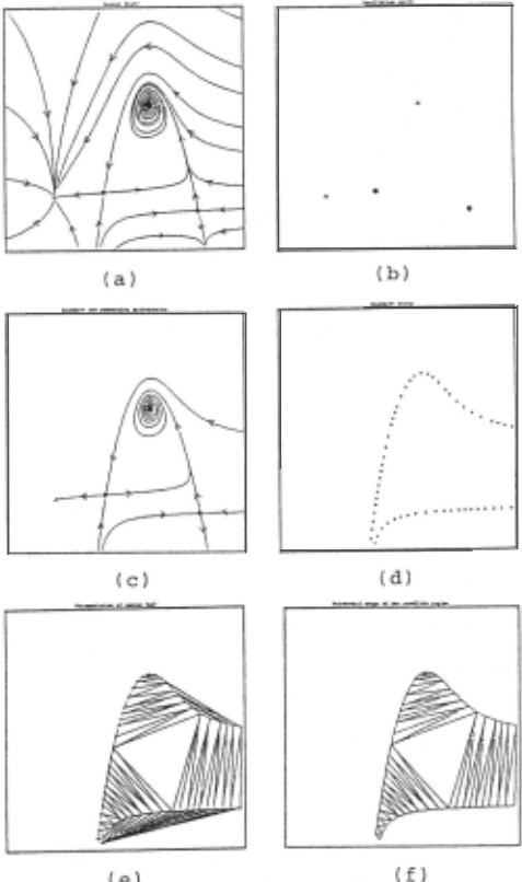
where u is a parameter. For the parameter value u = 0.2, the vector field within the region -1.0 ::; x ::; 4.0 and -1.0 ::; y ::; 4.0 is shown in Figure 3(a) . We use the algorithm to analyze the qualitative behavior of the system within this region.

The equilibrium points of the system are found by the Newton-Raphson method. MAPS locates four equilib­ rium points within the region and classifies their sta­ bilities by inspecting the eigenvalues of J acobians at the equilibrium points: two attractors at (0.0, 0.0952) and (2.0, 2.0) and two saddles at (1.05, 0.19) and

(3.05, -0.21), all shown in Figure 3(b) (attractors: +; saddles: Ef)). The stable and unstable trajectories of the saddle are then computed by integrating the system from a small neighborhood of the saddle in the directions of the stable and unstable eigenvectors backwards and for­ wards, respectively.

Since one of the unstable trajectories of each saddle goes to the attractor at (2.0, 2.0), the stability bound­ ary of the attractor consists of the stable trajectories of both saddles. Similarly, the stability boundary of the attractor at (0.0, 0.0952) consists of the stable trajecto­ ries of the saddle at (1.05, 0.19), one of whose unstable trajectories goes to the at tractor. However, within the region of interest there are trajectories that leave the bounding box. These trajectories can be conveniently thought of as the stable trajectories of an attractor at infinity. Therefore, the stable trajectories of the saddle at (3.05, -0.21) form the stability boundary for the at­ tractor at infinity, for one of the unstable trajectories of the saddle leaves the bounding box. Consistency rules are checked and satisfied. At the end of this step, MAPS finds three qualitatively different regions associated with the three attractors and internally represents the phase space structure in a data structure: the attractors are connected with each other via saddles and associated with stability boundaries (Figure 3( c)) .

The second step extracts a polyhedral approximation to each stability region preserving the gross features of the shape of the region. Consider the stability region of the attractor at (2.0, 2.0). The stability boundary is numerically approximated by a collection of trajectory points relatively uniform and dense on the boundary; see Figure 3(d) .

A Delaunay triangulation is performed on this set of points. As the result, the convex hull of the points is tes­ sellated with triangles; see Figure 3(e) . Under our condi­ tion that the points are reasonably dense and uniform on the boundary, the polyhedral shape of the stability re­ gion is contained in the triangulation of the convex hull. In order to extract the polyhedron, triangles exterior to the polyhedron have to be eliminated. We note two facts. First, the circumcircles of exterior triangles are larger than the circumcircles of the interior triangles [Boisson­ nat, 1984], since the interior triangles respect the local geometries of the boundary they approximate, whereas the exterior ones do not. Second, only certain type of tri­ angles are the candidates for elimination: the triangles with exactly one edge and two vertices on the bound­ ary of the convex hull in two dimensions. Therefore, we can focus the search and eliminate the exterior triangles by deleting the candidate triangle with the largest cir­ cumcircle, until the number of points on the boundary of the polyhedral approximation is the same as that of the original set of the boundary points or there are no more candidates for elimination (Figure 3(f)). We reit­ erate that the condition on the distribution and density of the boundary points has to be checked with respect to the shape of a region, to ensure that the circumcircle heuristic rule for elimination works.

MAPS compiles the data structure from step 1 into a relational graph, augments it with the polyhedral ap-

(e)

(f)

Figure 3: The analysis of a 2nd order nonlinear system: (a) vector field; (b) equilibrium points; (c) boundary and connecting trajectories; (d) points on the stability boundary for one of the attractors; (e) triangulation of the convex hull; (f) polyhedral approximation.

proximation, and reports to the user the following find­ ings:

<equilibrium-points:

1. saddle at:(3.05 -.21) 2. attractor at:(2. 2.) 3. saddle at:(1.05 .19) 4. attractor at:(O .. 0952)> <relational-graph: 1. stability-region for attractor at:·infinity·: stability-boundary: trajectory 1:(from ·infinity· to (3.05 -.21)) trajectory 2:(from ·infinity· to (3.05 -.21)) connecting-trajectories: trajectory 3:(from (3.05 -.21) to ·infinity·) 2. stability-region for attractor at:(2. 2.): stability-boundary: trajectory 4:(from ·infinity· to (1.05 .19)) trajectory 5:(from ·infinity· to (1.05 .19))

trajectory 1:(from ·infinity· to (3.05 -.21)) trajectory 2:(from ·infinity· to (3.05 -.21)) connecting-trajectories: trajectory 6:(from (1.05 .19) to (2. 2.)) trajectory 7:(from (3.05 -.21) to (2. 2.)) 3. stability-region for attractor at:(O .. 0952): stability-boundary: trajectory 4:(from ·infinity· to (1.05 .19)) trajectory 5:(from ·infinity· to (1.05 .19)) connecting-trajectories: trajectory 8:(from (1.05 .19) to (0 .. 0952))>

2.5 Other examples

We hav.e run MAPS on several other nonlinear examples, some with greater complexity and some of higher order.

The dynamical system for a buckling column under compressive force

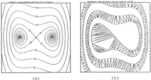
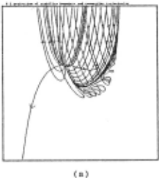
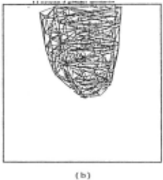
is a 2nd order system. For the parameter values a = -1.0, b = 2.0, and c = -0.2 and the phase space region -3.0 ~ x ~ 3.0 and -4.0 ~ y ~ 4.0, MAPS finds two attractors at (1.41, 0.0) and ( -1.41, 0.0) and a saddle at the origin, and generates a description of the phase space geometries: two banded stability regions associated with the two attractors, separated by the stable trajectories of the saddle at the origin. Figure 4(a) shows stability boundaries and connecting trajectories of two stability regions, and Figure 4(b) shows the polyhedral approxi­ mation to one of the regions.

Since the stability regions are interleaved, the geomet­ ric extraction algorithm using the circumcircle heuristic described earlier terminates before all the exterior trian­ gles are eliminated. A more expensive procedure is then used to eliminate the remaining exterior triangles: a tri­ angle is in a stability region of an attractor if the trajec­ tory starting at the centroid of the triangle approaches the attractor in the limit or enters another triangle al­ ready in the stability region.

Our algorithm works for higher dimensional systems as well. Consider the following 3rd order nonlinear system

MAPS locates an at tractor at (1.06, 0.0, 1.12) and a sad­ dle at ( -1.06, 0.0, 1.12) within the region -5.0 ~ x ~ 5.0, -5.0 ~ y ~ 5.0, and -5.0 ~ z ~ 5.0, and de­ termines that the stable trajectories of the saddle form the stability boundary for the attractor. The stability boundary is a two dimensional surface and is approxi­ mated by a set of relatively evenly spaced trajectories. MAPS then tessellates the phase space with tetrahedra and extracts a polyhedral approximation to the stability region of the attractor (see Figure 5).

3 Hierarchical Representation

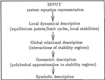
We have described and demonstrated our algorithm for analyzing a dynamical system through successive com­ putations on the system, starting from its system equation representation. MAPS generates a high level de­ scription of the dynamical system at the end of the analysis. To bridge the large semantic gap between the deduced symbolic description and the system equation representation of the input, we have employed multiple intermediate representations for the dynamical system, shown in Figure 6.

MAPS extracts the information incrementally, apply­ ing a set of operations to each intermediate representa­ tion. At each level of the representation, implicit prop­ erties of the system at different scales are made explicit and thus can be accessed and manipulated by the opera­ tors at the next level of the representation. In the order of analysis, MAPS generates a local description of equi­ librium points, limit cycles, and their eigenstructures, a relational description of equilibrium points, limit cycles, and their interactions, polyhedral approximations to sta­ bility regions, and a high level description of the phase space structure.

The internal representation of the phase space descrip­ tion as a relational graph captures the qualitative aspects of the phase space structure. In the relational graph, nodes are attractors and arcs denote the relations be­ tween their stability regions. Each node has informa­ tion about the attractor it represents, the associated sta­ bility region and its polyhedral approximation, and the boundary trajectories and boundary equilibrium points and limit cycles.

4 Related work

Yip has constructed a program, KAM, for automati­ cally analyzing Hamiltonian systems with two degrees of freedom in planar phase sections [Yip, 1989]. The program uses techniques from computer vision to clus­ ter point sets in phase sections and classifies phase por­ traits into meaningful categories. Our method applies to a large class of dissipative dynamical systems of any order in continuous phase spaces, in contrast to Hamil­ tonian maps on planar phase sections in KAM. Since we are interested in using MAPS to automatically syn­ thesize controllers in phase spaces, MAPS also extracts and represents stability regions with geometric pieces, as opposed to a point set representation in KAM.

Sacks' Poincare program analyzes planar systems through a partition algorithm on phase spaces and a bi­ furcation analysis on one parameter [Sacks, 1990] . The partition algorithm is based on the properties of two di­ mensional flows that do not .generalize to higher dimen­ sions. MAPS differs from Sacks' partition algorithm in that our method is able to analyze phase spaces of any dimensions, based on a general theoretical result on dy­ namical systems. MAPS generates a relational graph for a dynamical system characterizing the spatial arrange­ ment of phase space structures and containing geometric information about stability regions .

5 Conclusions

We have developed a qualitative method for automati­ cally analyzing phase space structures of nonlinear dy­ namical systems and have constructed MAPS to demon­ strate the method. MAPS looks at the phase spaces, finds qualitatively different regions-the stability re­ gions, and extracts and represents the qualitative fea­ tures. It employs deep domain knowledge about dynam­ ical system theory to recognize the qualitative structures of phase spaces. It computes a high level description of a dynamical system through a combination of numerical, combinatorial, and geometric computations and repre­ sents the phase space structure with a relational graph.

We are currently using our method to develop a novel control synthesis strategy for nonlinear control systems, with which a controller for a nonlinear system can be au­ tomatically synthesized in the phase space [Zhao, 1991b]. The strategy relies on the knowledge of phase spaces ob­ tained from MAPS, made possible by the internal rep­ resentation of the phase space structures. It generates control laws by synthesizing shapes of dynamical sys­ tems and planning and navigating system trajectories in the phase spaces. More specifically, the control strategy consists of a global control path planner and a local tra­ jectory generator. The global path planner finds optimal paths from an initial state to the goal state in the phase space, consisting of a sequence of path segments con­ nected at intermediate points where control parameter changes. The high-level description of the phase space is used to guide the search for the global paths. The local trajectory generator uses the flow information about the phase space regions to produce smoothed trajectories. Because of the human accessible aspect of the high level description, MAPS can also assist engineers in designing controllers for complex systems.