
Weak Equivalence for Constraint Sets
Proceedings of the Twelfth International Joint Conference on Artificial Intelligence. Logic Programming. Pages 851-855.
© 1991 International Joint Conferences on Artificial Intelligence
Abstract
We describe a generalization of equivalence between constraint sets, called weak equivalence. This new equivalence relation takes into account that not all variables have the same function in a constraint set and therefore distinguishes between restriction variables and intermediate variables. We explore the properties of weak equivalence and its underlying notion of weak implication with an axiomatic approach. In addition a complete set of axioms for weak implication is presented. With examples derived from the declarative rule language RL we show the applicability of weak equivalence to constraint solving.
- Denneheuvel, 1990
- S. van Denneheuvel & P. van Emde Boas, The rule language RL/1, A. M. Tjoa & R . Wagner ( eds. ), Database and Expert Systems Appli- cations, Proc. of the Int. Conf., Vienna, Austria, Aug, Springer Verlag Wien, 381-387.
- [Jaffar and Michaylov, 1987] J. Jaffar & S. Michaylov, Methodology and Implementation of a CLP System, Logic Programming, Proc. of the Fourth Int. Conf., Ed. Jean-Louis Lassez, 196-218.
- [Kwast, 1991] K. L. Kwast, The incomplete database, IJCAI'91, Morgan Kaufmann Publishers.
- [Leier, 1988] Wm. Leier, Constraint Programming Lan- guages: Their Specification and Generation, Addison- Wesly Series in Computer Science.
- [Vardi, 1988] M. Y. Vardi, Fundamentals of Dependency Theory, In: Trends in Theoretical Computer Science, Egon Borger (ed.), Computer Science Press, 171-225.
- [Van Emde Boas, 1986a] P. van Emde Boas, RL, aLan- guage for Enhanced Rule Bases Database Processing, Working Document, Rep IBM Research, RJ 4869 (51299).
- [Van Emde Boas, 1986b] P. van Emde Boas, A seman- tical model for the integration and modularization of rules, Proc. MFCS 12, Bratislava, Springer LNCS 233, 78-92.
- [Wolfram, 1988] S. Wolfram, Mathematica, A System for Doing Mathematics by Computer, Addison-Wesly.
References were extracted automatically from the PDF and may contain errors.
Full text extracted automatically from the PDF; figures, tables and equations may differ. The PDF is the version of record.
1 Introduction
Recently, constraint solving systems have emerged that allow declarative constraint processing (see for exam ple Mathematica [Wolfram, 1988], Bertrand [Leier, 1988] and CLP(~) [Jaffar and Michaylov, 1987]) whereas more traditional systems required user intervention to direct the solver towards a desired solution. From a general point of view, a typical input specification for these sys tems consists of a set of constraints and a set of restric tion variables which are "interesting" variables as far as the solver is concerned. The remaining variables in the set of constraints are intermediate variables. For con straint solving, restriction variables can be further di vided in two mutually disjunct sets, namely known vari ables and wanted variables.
Given the above input specification the objective of the constraint solver is to express all wanted variables symbolically in terms of known variables (i.e. with out supplying actual values for the known variables). In such a symbolic solution only restriction variables are allowed and as a consequence all intermediate vari ables must be eliminated from the input constraint set. As a simple example consider the input constraint set { .r = y + 2, y = z + 2} where z is known and .r is wanted, so .r and z together are the restriction variables. A con straint solver set to solve this problem will probably re turn { .r = z + 4} as the solution, thereby eliminating the intermediate variable y. For such a solver output, we would like to say that it is in some way equivalent with the input constraint set. Unfortunately the standard definition for equivalence among constraint sets would classify the example input and output as inequivalent, since the output set does not impose any restriction to the intermediate variable y.
Therefore we define a more general equivalence, called weak equivalence which distinguishes between restriction variables and intermediate variables.
2 The rule language family RL
Our primary motivation for investigation of weak equiv alence lies in its role in the integration of relational databases and constraint solving. This integration is one of the aims of the rule language family RL (see [Van Emde Boas, 1986a, Van Emde Boas, 1986b]). In the RL languages, knowledge can be represented in three differ ent types of rules: tabular rules, clauses and constraints. Corresponding to these types of rules there are three ar eas of technology that support that style of knowledge processing in isolation: Database Systems, Logic Pro gramming Systems, and Spreadsheets. A main goal of RL is to integrate these three technologies in one knowl edge base system. Query processing should be executed with the help of an existing relational database system; knowledge and queries expressed in RL are to be pre processed by a constraint solver, and to be compiled into a database query language so that large amounts of data can be processed effectively.
In the current prototype of RL/1 we focus on the inte gration of a constraint solver with a relational database system; RL/1 has been presented elsewhere [Den neheuvel, 1990]. The RL/1 prototype system has been implemented in Prolog which includes a language parser, a database system and a constraint solver. The examples presented in this paper were processed success fully by this prototype.
Terms in RL/1 are constructed inductively in the usual way from constants, variables and functions. Both numeric and string domains are supported. For use in the database application we include binary functions such as+, -, * and /. Constraints include expressions of the form t 1 op t 2 with opE { =, >,<,::f.,~.~} and two special constraints false and true. Null values are not available in the language itself but may be present in the tables of the underlying database (cf. [Kwast, 1991]).
In RL/1 a distinction is made between extensional objects and intensional objects. Extensional objects correspond to base tables in the underlying relational database. Intensional objects on the other hand are ob jects whose relations can be materialized by evaluation of their definition. An intensional object is defined by one or more rules, alternatively called clauses. A rule typically consists of a rule head and a rule expression separated by the keyword WHEN. The rule expression contains constraints or invocations of intensional and ex tensional objects, separated by the conjunctive AND op erator. Defining an intensional object with several rules expresses disjunction between the rules. The question whether a rule expression as a whole denotes a finite or infinite relation is in general undecidable; partial in formation about this question is obtained from the con straint solver.
2.1 Query commands
Query commands in RL /1 result in an answer relation which consists of attributes and a (possibly empty) set of tuples. Optionally the result of a query command can be stored in an extensional table object. There are the following types of query commands:
liFER ( attribute-list ) WHEI rule-exp [ TO table ] SHOW rule-exp [ TO table ]The INFER command yields an answer relation with attributes equal to the attribute list between the INFER and WHEN keywords. The SHOW command yields an answer relation whose attributes are the variables occur ring in the rule expression.
Processing the above queries requires one or more in vocations of the constraint solver. The solver output is used to compile the query into a database request. Sym bolic queries on the other hand work by presenting this intermediate solver output to the user directly:
The 'TO file' option allows the computed symbolic answer to be stored in a text file. Symbolic query com mands produce one or more of the following answers:
condition= Condition set solution= Solution set
The solution set contains elements of the form x = t with x a wanted variable and t a term. The terms t in the solution set contain only known variables. The condition part consists of constraints over the known variables; it states under what additional restrictions the obtained solution is valid. Intermediate variables are eliminated from both the condition and the solution set. Known variables are determined by the rule expression of the query and wanted variables by the attribute list of the query.
3 Symbolic computation in RL/1
Intensional objects are declarative representations of knowledge; therefore it is not known beforehand how the attributes of an object are invoked. For instance con sider the module in Figure 1 for a parallel circuit of two resistors. In the representation of the circuit both the physical laws of basic electricity theory and the practi cal condition that the resistors should not be overloaded are expressed in terms of constraints. We know from elementary physics that the values given in the table ex perimentdata fully determine all quantities. How should the RL/1 knowledge base determine that this is indeed the case? The constraint solver is capable to figure out the determinedness.
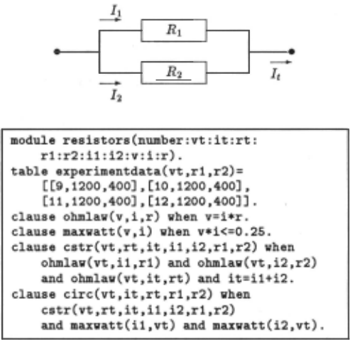
Suppose voltage is applied to the example circuit then the current through the circuit and the total resistance can be calculated:
With other variables given, an answer is also computed:
In the constraints for the circuit the law for parallel resistors is not given directly, but the total resistance rt can nevertheless be computed. Now suppose we ap ply various voltages to the two resistors as specified in the experimentdata table in Figure 1. In the experiment the voltage is slowly increased and the resistors stay the same. Surely at some high voltage the circuit will break down. Let's run the experiment (the '(*)' notation ex pands to all attributes of the involved object):
| show vt | experimentdata(•) rl | r2 | rt | and eire(•) it |
|---|---|---|---|---|
| 9 | 1200 | 400 | 300 | 0.03 |
| 10 | 1200 | 400 | 300 | 0.033 |
In the answer relation the rows are corresponding to the rows from the experiment data table but obviously some rows are missing. In these missing rows the con straints were not satisfiable (i.e. the non-smoking condi tion maxwatt(i2,vt) was violated) so they do not appear in the answer to the query.
The capability to produce symbolic output is an im portant feature of the RL/1 knowledge base. It allows the user to analyze relationships between variables and to infer relationships that hold in special circumstances. A general relationship between the resistance of the indi vidual components and the total resistance can be found with the following symbolic query:
syminfer(rt) when known(r1,r2) and cstr(*) solution= rt=r1*r2/(r1+r2)The constraint solver has inferred the law for parallel resistors.
The classification of variables in the three disjoint par titions of wanted, known and intermediate variables is crucial for derivation of relationships like the previous example. By making r 1 and r 2 known and r 1 wanted the constraint solver of the RL/1 system was directed to wards a solution that expresses r1 in terms of r 1 and r 2 · The constraint solver actively applies this information in its inference process to yield the desired result.
On the other hand suppose that variables of a con straint set were classified in only two partitions of wanted and intermediate variables as is the case in many existing constraint solving systems. The constraint solver would correctly establish that the equation system is undeter mined (there are too many variables and not enough equations to solve them).
In the next sections we formalize the notion of equiv alence that is used by the solver.
4 Weak equivalence and implication
First we introduce some definitions and notations. Vari able names are chosen from non capitals (x, y, z, .. . ) and sets of variables from capitals (X, Y, Z, .. . ). V is the set of all variables. Constants are denoted by c and functions by f. Terms are denoted by t. Sets of constraints are represented as A, B, Cor D. To denote the cardinality of a set I we use the notation 11111.
Solutions are constraints of the form x = t with x fl. var(t). The variable xis called the head variable and the variables in the term t the tail variables.
Definition 1 A solution set is a finite set {x1 = tt, ... , Xn = tn}, satisfying: 1. ll{xt, ... ,xn}ll = n, (the variables are distinct} 2. {x~, ... ,xn}nvar({t~, ... ,tn}) =0Definition 2 A tuple is a solution set of the form { X1 = c1, ··· , Xn = Cn} with Ct, ... , Cn constants.Solution sets are denoted by~.~ and E> and tuples by ¢, t/J and 8. For a solution set~= {x1 = t~, ... , Xn = tn} the head variables x1, ... , Xn are denoted as hv(~).
The operator restrict retains those solutions in ~ that have a head in X:
Solution sets ~ = { x1 = t1, ... , Xn = tn} can be in terpreted as substitutions [x1 := t1, ... , Xn := t,] which can be applied to (collections of) items:
A tuple ¢ satisfies constraints in A, ¢ f= A, if and only if ¢ satisfies all constraints in A. A set of constraints A implies a set of constraints B, A ~ B, if¢ satisfies B whenever ¢ satisfies A, for all tuples ¢.
Definition 6 (Strong equivalence) 1. ¢ f= A iff 'Va E A(¢ f= a) 2. A~ B iff 'V¢ (¢ f= A=>¢ f= B ) 9. A = B iff A ~ B & B ~ AIn the case of weak equivalence these definitions are subscripted with the restriction variables X. The notion of strong satisfaction is changed to weak satisfaction by existentially quantifying the variables not in X (i.e. the intermediate variables). As a consequence the values of these variables in the tuple ¢ are no longer involved in the satisfaction of A.
Definition 7 (Weak equivalence) 1. ¢ F x A iff 3t/J ( t/J F A & ¢ = x t/J) 2. A ~x B iff 'V¢ (¢ f= A=>¢ f=x B) 9. A =x B iff A ~x B & B ~x A Example 1 (Equivalence) {x = 1} =f:.x,y {y = 1} {x <X+ y, y > 0} =x true {x = 1} =f:.x {y = 1} {x < x + y, y > 0} =Y {y > 0} {x=y}=x{x=z} {x<x+y,y>O}={y >O}In the above definitions we presented strong impli cation between constraint sets as an implication using strong satisfaction in both the premise and the conse quent. Weak implication was constructed from this def inition by weakening the consequent of the implication to weak satisfaction. It may be conceivable that other interesting definitions arise if instead only the premise of the implication is weakened (single implication) or if both the premise and the consequent are weakened ( dou ble implication):
Definition 8 (Single and double implication)
In the next proposition we compare these four possible definitions of implication.
Proposition 9 (Relating implication definitions)
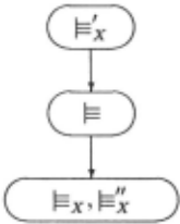
1. A ~'x B =>A~ B (A~ B ~A ~'x B) 2. A~ B =>A ~x B (A ~x B ~A~ B) 9. A~; B {:}A ~x BThe relationships between the four definitions are summarized in Figure 2 (arrows denote implication). Single implication is too strong and only applicable when var(B) C X, in which case it is equivalent to strong implication. Double implication is equivalent to weak implication and therefore superfluous.
4.1 Inconsistency, tautology and redundancy
Inconsistency is normally defined as strong equivalence with the special constraint false. As a consequence tau tology and redundancy can be defined in terms of strong and weak equivalence. The strong definitions are ob tained from the weak definitions by dropping the sub script X.
Definition 10 (Strong and weak inconsistency)
- Incx(A) iff A =x false
2. Tautx(A) iff A =x true
3. Redx(A) iff 3B C A (IIBII < IIAII & A =x B)
It turns out that weak and strong inconsistency are ac tually equivalent:
Proposition 11 1. A I= x false '¢> A I= false 2. A =x false -¢> A = false- Inc(A) -¢> Incx(A)
However, contrary to inconsistency, weak tautology is truly weaker than strong tautology:
Proposition 12
- Taut(A) => Tautx(A)
- Tautx(A) ::/;> Taut(A)
It is easy construct a counter example such that Tautx(A) but not Taut( A). Let A= {x < x + y, y > 0} then it holds that {x < x + y, y > 0} ={r} true so Tautr(A). On the other hand -,Taut(A) because {x < x + y, y > 0} := {y > 0} t=. true.
As a consequence weak redundancy is not equivalent to strong redundancy:
Proposition 13
- Red(A) => Redx(A)
- Redx(A) ::/;> Red(A)
Again we can construct a counter example such that Redx(A) but not Red(A). Let A = { x = y+2, y = z+2} then it holds that A ={r,y} {x = y+2} so Redx(A). On the other hand -,Red( A) because both { x = y + 2, y = z +2} t=. {x = y+2} and {x = y+2,y= z+2} t=. {y= z + 2}.
5 Weak axioms
In this section we enumerate axioms that hold for impli cation and equivalence. We start with some properties of strong implication that are maintained for weak im plication.
Proposition 14 (The equivalence relation =x)
1. A l=x A 2. A I= x B & B I= x C => A I= x C 3. A =x A 4· A =x B => B =x A5. A :=x B & B =x C => A :=x C
Now we explore some axioms that are specifically con cerned with the restriction variables of weak implication. As was to be expected, restriction variables can be harm lessly deleted:
Proposition 15 (Removal of restriction variables)
1. A I= xuY B => A I= x B- A :=xuY B => A =x B
A variable can be added to the set of restriction vari ables X in A I= x B if it does not occur in B:
Proposition 16 (Addition of restriction variables)
1. A l=x B =>A l=xuY B if var(B) nYC X
2. A =x B =>A =xuY B if var(A U B) nYC X
For strong implication we have, among others, the fol lowing axioms:
Proposition 17 (Axioms for strong implication)
- 1.AUBI:==A
2. A I= B & A I= C => A I= B u C
9. A I= B => A U C I= B U C
- A I= B u C =>A I= B
5. A I= B & B u C I= D => A u C I= D
6. A I= B u C & B I= D => A I= C u D
7. A I= B & C I= D => A u C I= B u D
The axioms (1) and (2) are known in Functional De pendency Theory [Vardi, 1988] as decomposition and union respectively. From these axioms and transitiv ity (axiom (2) of Proposition 14) all other strong axioms (3)-(7) can be derived. For weak implication however the situation is different, since only ( 1) and ( 4) hold un conditionally:
Proposition 18 (Axioms for weak implication)
1.AUBI:==xA 2. A I= x B & A I= x C => A I= x B U C if var(B) n var(C) c X 9. A I= x B => AU C I= x B U C if var(B) n var(C) C X 4· Al:==xBUC=>AI=x B 5. A l=x B & B U C l=x D =>Au C l=x D if var(B) n var(C) C X 6. A l=x B u C & B l=x D =>A l=x CuD if var(C) n var(D) C X 7. A I= x B & C I=-} D => A U C I= x B U D if var~B) n var(D) C XThe conditional axioms of Proposition 18 are more general than their counterparts in Proposition 17 since from the conditional axioms the unconditional axioms can be derived. For instance axiom (2) in Proposition 17 can be derived from axiom (2) in Proposition 18 by as signing to X the set of all variables V in which case the condition becomes trivially true.
| Name | Ax10m | Restnct10n |
|---|---|---|
| True False Weakening Transitivity Union Substitution Generalization Abstraction Removal Irrelevance | A }=x true false l=x A AUBI=xA A l=x B & B l=x C => A l=x C A l=x B & A l=x C => Al=xBUC AU~I=x~(A)U~ ~(A)U~I=xAU~ ~(A) l=x AU~ Al=~yB => A l=x B A 'X B => A l=xuY B | var(B) n var(C) C X hv(~) nx = 0 var(B) nYC X |
The proof of the proposition is added to illustrate the convenience of reasoning by means of weak equivalence.
8 An elaborated example
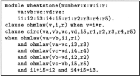
As an illustrative example of application of weak equiv alence consider the circuit of Figure 4 derived from the domain of electronics. The corresponding RL/1 repre sentation is listed in Figure 5. In ancient history the bridge of Wheatstone was used to measure ohm resis tance. In the setup, r 1 (or r2 ) is a variable resistor and r4 (or r3) the unknown resistor. The component in the center is an ampere meter with resistance r 5 . For measurement the variable resistor is adjusted so that no current flows through r 5 . In this balanced state the fol lowing relationship holds:
To see if theory matches reality we apply 10 volt at the clamps of the circuit. In case we choose the values of the resistors all equal to 200 ohm then the circuit is in balanced state and the RL/1 knowledge base can compute the values for Vb, Vc and i5:
To obtain this answer, the solver infers the following weak equivalence:
6 Completeness
A natural question that arises in the context of an ax iomatic approach is whether a sound and complete ax iomatization is feasible. As a first step we proved the soundness of all axioms in Figure 3.
Proposition 19 For general constraints, the axioms in Figure 3 are sound.
Both for weak and strong implication, a completeness result can be derived. We proved completeness with re spect to primitive constraints, that is constraints of the format 'x = y' or 'x = c':
Proposition 20 For primitive constraints, the axioms in Figure 3 are sound and complete.
For completeness the axioms concerned with substitu tion have to be added to the ones we gave before. The most interesting axiom is Abstraction that allows you to add solutions for intermediate variables.
From the complete set for weak implication a complete set of strong axioms can be easily inferred. Abstraction is never applicable for strong implication so it is replaced by the derived axiom Instantiation:
7 Constraint elimination
Intuitively more constraints can be eliminated if weak equivalence is used instead of strong equivalence. In this section we provide a proposition that specifically exploits weak equivalence for constraint elimination. A subset B of a set of constraints A U B is redundant with respect to the restriction variables if there exists a solution set ~ for intermediate variables such that ~(B), the effect of substituting ~ on B, is equivalent with true:
Proposition 21
A U B =x A if there exists some ~ such that: 1. ~(B)= true 2. hv(~)nX = 0 3. hv(~) n var(A) = 0 Proof: i) AU B l=x A: Weakening. ii) A l=x AUB: A l=x A =>A l=x ~(A) .................................... (3)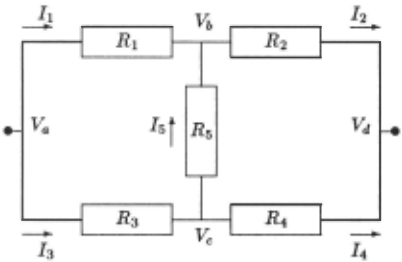
If one of the resistors, say r 1, is taken larger than the others, a small positive current flows through the center resistor:
It might be quite interesting to see if the relationship for r 4 can be inferred symbolically from the represented knowledge under the assumption that the circuit is in balanced state. We want to express r4 in terms of r1. r2 and r3 so these latter variables are specified as known variables. As an extra constraint we know that since the circuit is in balanced state no current flows through rs:
syminfer(r4) when eire(*) and i5=0 and known(r1,r2,r3). solution= r4=r2*r3/r1To obtain this answer, the solver had to infer the follow ing weak equivalence:
{ Va - Vb = i1 * r1, Va - Vc = i3 * r3, Vc- Vd = i4 * r4, vb- Vd = i2 * r2, Vc- Vb = is* rs, i1 +is = i2, i4 +is = i3, is= 0} ={r1 ,r2 ,r0 ,r4 } {r4 = r2 * r3/rdThese equations are nonlinear by the occurrences of the terms i 1 * r1, i2 *r2, i3 * r3, i4 *r4 and is *rs (note that the known variables r1, r2 and r3 are in fact not given as a value and therefore contribute to the nonlinearity of the constraint system).
9 Conclusion
In this paper we used weak equivalence to express, ex plicitly, the functional difference between wanted, known and intermediate variables in a set of constraints. By a complete set of axioms we established the main proper ties of weak equivalence. Using these axioms we proved an application independent tool to simplify constraint sets using this new form of equivalence.
With examples run on a prototype implementation we showed practical applicability of weak equivalence for constraint solving purposes. By distinguishing wanted, known and intermediate variables in a constraint set the solver can be guided towards a solution that discards in termediate variables and expresses wanted variables in terms of known variables. Derivation of symbolic rela tionships is facilitated by the theoretical concepts intro duced in this paper in two ways. Firstly, weak equiva lence allows you to express formally the correspondence between the derived relationship and the original con straint set. Secondly the reasoning necessary for in ference of symbolic relationships can be represented in terms of weak equivalence.
@inproceedings{ijcai1991p125,
  title     = {Weak Equivalence for Constraint Sets},
  author    = {van Denneheuvel, Sieger and Kwast, Karen L.},
  booktitle = {Proceedings of the Twelfth International Joint Conference on
               Artificial Intelligence, {IJCAI-91}},
  publisher = {International Joint Conferences on Artificial Intelligence},
  editor    = {John Mylopoulos and Ray Reiter},
  pages     = {851--855},
  year      = {1991},
  month     = {8},
  note      = {Logic Programming},
  url       = {https://ijcai.org/proceedings/1991/125},
}
TY - CPAPER TI - Weak Equivalence for Constraint Sets AU - van Denneheuvel, Sieger AU - Kwast, Karen L. T2 - Proceedings of the Twelfth International Joint Conference on Artificial Intelligence, IJCAI-91 PB - International Joint Conferences on Artificial Intelligence PY - 1991 SP - 851 EP - 855 UR - https://ijcai.org/proceedings/1991/125 ER -Copied
Machine-readable versions of this paper, for tools and AI agents:





