Learning to Diagnose by Doing

1 Introduction

A_ complex pro~lem-solving task generally allows for many d1ffe~ent strategies, all of which could potentially lead to a solutio~. H?wever, all the strategies are not equivalent. They differ m terms of their efficiency in arriving at the solution, the cognitive load they place on the problem­ solver and the generality with which they can be trans­ formed to other problems. For someone encountering a task for the first time, some strategies might become apparent immediately and others become apparent more slowly as the proble~-solver becomes familia_r with the task. The process by wh1ch a person who begms a task with "obvious" strate~ies, gr~d_ua~s ~o more efficient strategies with in­ creasmg fam1har1ty IS what we call learning or skill acquisition I.

In this paper, we are interested in understanding this pro~ess for a cla_s~ of problem-solving tasks called diag­ nosis. ~ore spec1f~c~ly we foc~s our attention to diagnosis of machmes. Intwt1vely machmes are defined as devices designed to fulfill a function. If such a device produces aberrant b~havio~, w_e arc inte~ested in identifying that part of the ~ev1ce ~h1ch .'s rc~pons1ble for such behavior. Typi­ cally, diagnosis begms wllh a model of the device and a set of symptoms indicative of aberrant behavior. This model is Eswaran Subrahmanian Engineering Design Research Center Carnegie Mellon University Pittsburgh, PA 15213

*This research was funded by NSF Grant IRI-8807061

1 The thread of the argument in this paper is inspired by [Anzai and Simon, 1979]

a description of the structure and behavior of the device. Given this information, there are many strategies available for diagnostic problem-solving. We are interested in the learning process that occurs in this problem domain.

2 The Learning Task

In t~is paper, we have chosen an abstract example of a diag­ nostic problem. Although this example is limited in some o~ it's as~umptions .· it is g~neral enough to be applicable to a w1~e vanety of d1agnosuc problems. The results in this article ar~ ~ased on .a longitudinal study of a single subject. The empmcal base 1s a protocol of the subject as he solved this problem until he mastered the most sophisticated strategy. Based on an analysis of the protocol [Ericsson and Simon, 1980], we have identified four different strategies that were used by the subject to solve the given set of problems. These strategies vary in their efficiency of diag­ nosis and in their modes of reasoning. We also analyze the protocols to identify the different operators that were used by the subject to transform one strategy into a more efficient one.

We have characterized each strategy in terms of produc­ tions in an effort to indicate how it could be simulated on a computer. Similarly, we characterize the learning operators based on the cues used by the subject to provide an account of the transformation of a strategy to a more efficient one.

3 Method

The experiment was carried out in two sessions. The first session lasted about 30 minutes and the second one lasted about 45 minutes. The subject is an adult male, a graduate student at the business school at Carnegie Mellon. The subject was ~amiliar with networks and their analysis prior to the expenment although he was not familiar with the par~cular set of problems that were posed to him. Each sess10n consisted of solving eight problems. The network for each problem is identical but the set of observed symptoms are different.

The subjected was instructed to think aloud while solving the problems. The protocol of his verbalizations were recorded on tape and later transcribed. The instructions for the problems were as follows:

The task involves fault diagnosis of graphically dis­ played networks. These networks operate as follows. Each component has a random number of inputs. Similarly a random number of outputs emanate from each component. Components are devices that produce either a 1 or 0. An output of 1 denotes an acceptable output; 0 denotes an unacceptable output. All outputs emanating from a component carry the value produced by that component.

A component will produce a 1 if:

1. All inputs to the component carry values of 1 and

2. The component has not failed.

If a component fails, it will produce values of 0 on all outputs emanating from it.

A problem begins with the display of a network with the outputs indicated (refer to Figure 1 for an example). Based on this evidence you are asked to identify the failed component In order to perform this task you are allowed to test connections between components but minimize the number of measurements you perform. Keep in mind that only one failed component can explain the given set of readings.

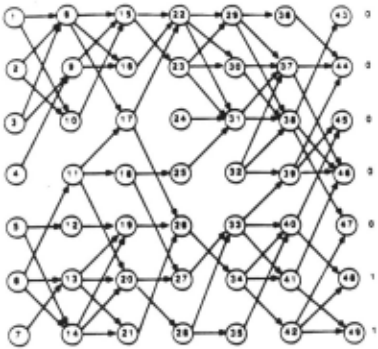
Each session consisted of solving eight problems. As stated in the instructions, the network for each problem is identical but the set of observed symptoms are different

Unlike in physics problems we do not have available (for this task) any characterizations of the expert and novice be­ havior. Therefore we need a measure to compare the perfor­ mance of novices and experts. Since for this particular task, we indicated that expertise is understood in tenns of problem solving efficiency, we propose to use the number of measurements as a metric for comparing perfonnance. The cost of of all measurements have been assumed to be equal. The network problems of the size we use can be solved for optimal solutions. We shall measure the perfor­ mance on a given task in relation to the optimal possible perfonnance.

4 Results

The protocol consists of a total of 280 statements divided into two sessions. In this paper, the set of eight problems in each of the two sessions are numbered P1 - P16. Problems P1 through P8 belong to session 1, and P9 through P16 to session 2. The first session consists of 104 statements and the second 176 statements. Session 1 contains 52 state­ ments about measurements between connections, 21 per­ taining to reasoning to identify the next component or set of components that could be faulty, 7 metastatements about strategy, 4 verifications of faults, and the rest are obser­ vations and conjectures; Session 2 contains 41 measure­ ments of connections, 79 pertaining to reasoning to identify the next component or set of components that could be faulty, 25 metastatements about strategy, and the rest are observations, explanations and conjectures.

The protocols for both the sessions are explicit enough to leave no doubt about the strategy that is being used by the subject at any given moment However, the protocols are not sufficiently complete as to identify how the subject ac­ quired or used infonnation to transfonn his strategy. This lack of explicit evidence for the process of adaptation is also reported by [Anzai and Simon, 1979]. The rest of the analysis is based on the four strategies developed by the subject to solve the problems.

4.1 Depth-First Strategy

The strategy that the subject used P1 - P7, except P5 is what we call the depth-first strategy. From the problem defini­ tion the subject hypothesized correctly that a faulty com­ ponent has all inputs as 1 and all outputs as 0. The search for a faulty component was not random. He chose the frrst 0 (from the top) for a given set of outputs and checked for it's inputs. If one of the inputs was a 0, then he concluded two things: (a) The component under consideration is not faulty and (b) the faulty component could be traced to the component whose corresponding output was 0 or a com­ ponent before that. This strategy always leads to the solu­ tion and restricts the search to one component at any step. At each step, through extensive testing only those com­ ponents with output 0 are explored. However, this strategy is non optimal in the number of measurements perfonned. For example, problem 1(P1) in session 1 required 6 measurements, whereas optimally it can be solved with at­ most 3 measurements.

While solving each of these problems, the subject verified his result by tracing the outputs of the faulty component to the 0 outputs at the tenninal nodes. For example in P2 he traces the output of the faulty component (32) to all the tenninal nodes with 0 outputs (43, 44, 45, 46, 47). We present a section of his protocol to illustrate this:

17.S:there are no inputs into 32, then 32 is at fault! 18.S:that should explain all the other zeroes, let's see, 37 has output 41, it that a 0 [yes]

19:S:37 to 46? [a 0] 20.S:32 to 39? [a 0] 21.S:39 to 45 must be a 0, and 39 to 46 must be a zero and 38 to 47 must be a 0 22.S:okay 32 is at fault!

From solving this set of problems the subject retained two pieces of infonnation in the long-tenn memory. These are: (a) a faulty component has all inputs as 1 and outputs as 0, and (b)the outputs from a faulty component can be ul­ timately traced to the 0 outputs at the tenninal components.

In figure 2, we provide a set of productions which can simulate this strategy2.

In enumerating the productions, we have assumed that we have a structural description of the network available. This implies that for any given node:

ZWe enumerate only those productions which are vital for explicating each strategy

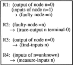
• All the predecessor and successor nodes can be generated. Hence functions like find-inputs are capable of generating all nodes which have in­ puts to a given node. Similarly, the nodes con­ nected to the outputs of a given node are avail­ able and hence functions like trace-output can apply recursively to find paths from a given node to the terminal nodes. These functions have not been described here.
• The value of the connections between any two nodes can also be checked. Functions like input and output can check if the value of the output from a node, or the values on the input of the node are 0, 1 or unknown.

From the defmition of the productions, the reader can verify that this executes the depth-first strategy.

4.2 Refined Depth-First Search

The strategy used during this episode is what we call the refined depth-first strategy. This strategy was used for only problems PS, P8, P9 and ~10 .. This indicates that the s~bject remembered this strategy m h1s long-term memory which he was able to recall later.

This strategy is similar to the depth-first strategy in ~at the subject begins the search from the first component w1th output 0 (from top, refer to figure 4-1). For this component he identifies all the inputs and their corresponding com­ ponents. At this point, he departs from depth-first. Inst~d of measuring each input, he picks one component at a ume (generally top to bottom) and traces the output of that com­ ponent to all the terminal nodes. If none of the components have outputs that trace to all the terminal Os, then he picks the first component and generates all the inputs. The sa~e procedure is continued. However, when a component lS identified whose output traces to all the Os, then he measures the inputs and the outputs to verify that the com­ ponent is faulty. When the above strategy is followed it always leads to the correct solution and even though the number of measurements is less than the "depth-first strategy", they are not minimized.

The subject first used this strategy for PS and then for P8. In both these problems all the terminal nodes are 0, which prompted him to remember at each step, that any component under consideration has to ultimately explain all the ter­ minal Os. He also used this strategy for P9, P10. He clearly states this strategy while solving P9: "so basically my strategy is to locate that node from where there are paths to all five (terminal Os), ... ".

The main piece of information retained in this stage is a perceptual one. As the subject traced the outputs of suspected candidate, he discovered visually that a path from a given node to a terminal node is equivalent to a path from a terminal node to a given node in the network. The productions for this strategy are shown in figure 3.

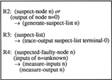
The productions in figure 3 similar to the one's for depth­ first. The production R1 is common to all strategies. For each strategy the productions that are presented are replace­ ments of the productions with the same number in the pre­ vious strategy. For example, the production R2 in ~e "refined depth-first" is intended as a replacement of R2 m the "depth-first". The function generate-suspect-list provides a list of components which feed inputs into a gi~en node. This list is called "suspect-list". The function trace-output is the same as before. If it succeeds for any node on the suspect-list it is returned as a "suspected-faulty­ node" else it returns the first node on the "suspect-list" which triggers R2 to recurse. Once the suspect is isolated, R4 triggers measurements.

The control structure for this strategy is as follows: Once a suspect-list is generated, it becomes the immediate goal. This ensures that the suspect-list of the first 0 is explored. Similarly, as soon as R2 generates a suspected-faulty-node or a suspect-node, these are treated as immediate goals which take precedence over other productions.

4.3 Simultaneous Propagation

The use of the "simultaneous propagation" strategy is first apparent in P11. This strategy involves tracing the inputs of all the terminal nodes with 0 outputs, one level at a time. Once the input components for each terminal 0 are iden­ tified, the subject checks to see if there are one or more components which are common to all sets of inputs. If such a node(s) is found, then a faulty component is identified. It is only after identifying such a root node that any measure­ ments are made. If a root node is not identified at a given level, then all the inputs to each of the suspect components are generated and the same check is performed, else if a single root node is identified then the subject measures the inputs to verify that it is indeed the faulty component. ~fa set of nodes are identified, then the outputs are frrst measured to identify which component in the set produces a 0 output. Once this is done the inputs are measured to verify the faulty component. This strategy minimizes the number of measurements.

This strategy is clearly and succinctly stated by the sub­ ject in P13: "I just trace the arcs backwards from the nodes I want (terminal Os) and see if they converge at some point (node) someplace". The subject also solved Pll,Pl2 and Pl3 using this strategy. The productions for this strategy ace provided in figure 4.

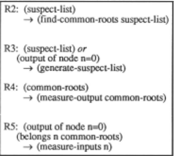
The control structure here is slightly different from pre­ vious strategies. When R2 is fired and a suspect-list is produced, this list is not marked as an immediate goal. In­ stead the input components of all the nodes with Os ace generated in the suspect-list, which is a list of lists. Only when all Os ace exhausted does R2 fire again. The function find-common-roots finds all the nodes common between all the lists of the suspect-list. If there is none, then R3 is fired and recursed to the next level. However, if common-roots ace found then the inputs and outputs are measured to iden­ tify the faulty component

4.4 Refined Simultaneous Propagation

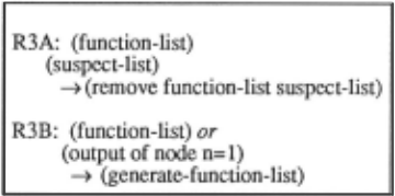
This strategy is very similar to simultaneous propagation. The only difference is the fact that each step some ad­ ditional information is used to eliminate some of the suspects. We call this refined simultaneous propagation. This strategy is also optimal in the number of measure­ ments, but is computationally more efficient since some of the suspects ace eliminated at each step.

In this strategy, as before, the inputs to each of the ter­ minal nodes with a 0 output are identified. Simultaneously all the input nodes with terminal 1 are also traced. Since all the inputs to a node with output 1 should be functioning normally, the corresponding nodes ace eliminated from each list of suspected faulty components. This reduces the num­ ber of suspects that need to be examined at each step. Once this done, the subject examines the suspect-list to determine if there ace one or more components which are common to all the suspect lists. If none is found, the same procedure is repeated at the next level and so on. Only when a root node(s) is identified ace any measurements made.

The first use of information from an output of 1 is in­ dicated in Pl4. The explanation for this is provided in protocol, a segment of which we provide below:

105.S: That means the node I am looking for cannot be 38 or any nodes that precede 38. 106.S: Because 38 has an input into to 43 and also other nodes, and 43 shows a 1.

This strategy is also used in Pl6, but since PIS has all Os at the terminal nodes, the subject could not use this strategy.

To characterize the strategy described, two productions R3B and R3A (figure 5) are added to the list from the "simultaneous propagation" strategy. R3B generates the list of components that are functioning properly, and R3A removes these components from the suspect list.

5 Learning

In the preceding sections, we characterized four different strategies that the subject used to solve the diagnostic problem. We also showed that the subject started with the simpler strategies and over time evolved to using more sophisticated strategies. This is the learning process. We have yet to indicate how this process occurs. In this part of the paper, we provide a description of how the subject moves from one strategy to another based on the protocol.

As we noted before, the subject when presented with the first problem began solving it immediately. This search is far from random and suggests that the subject has available some prior knowledge of some general problem-solving strategies. As he solves problems he is able to gather new information which he combines with his prior knowledge to improve his problem-solving strategies. This implies that the subject has also available some learning capabilities in his long-term memory.

In this section we describe four ways in which the subject combined new knowledge with prior knowledge to improve his problem-solving skills. From the protocol we have iden­ tified the different pieces of information which provided the subject with cues to develop new strategies. We also provide operators which combine this new information with prior knowledge to produce new strategies.

5.1 Knowledge from Depth-First Search

In the depth-first strategy, the subject used two characteriza­ tions of a faulty component. First the subject realized that a faulty component has inputs that ace all 1 and outputs that are 0. Another necessary condition for a component to be faulty is that it's inputs should lead to all the terminal nodes with a 0. The subject started by using the first definition as a goal for search. But as is apparent, this strategy requires extensive measurements. After he located the faulty com­ ponent, he used the second characterization to verify his hypothesis.

The two characterizations are equivalent in terms of their ability to guide the search to the correct solution. However, using only the first defmition (of a faulty component) is not optimal in terms of the number of measurements required to reach a solution. The subject realizes that the use of the second definition does not require any measurements to identify a faulty component and it would be more efficient to use this definition to check for each suspect before making any spurious measurements.

This learning process can be implemented simply in terms of re-ordering the firing of productions (Figure 2). For any given node with output 0, R3 fires and generates all nodes with outputs leading to the given node. Each of these nodes are potentially faulty. In the depth first strategy, the outputs of each of these are measured to identify which node might have a 0 output. This is done by firing R4. Instead one could fire R2 to check if any of the nodes can explain all Os. Hence flipping the order in which R4, R2 fires leads to a more optimal solution. This process provides the mechanism by which the transition from depth­ first to refined depth-first occurs.

5.2 Knowledge from Refined Depth-First

During the stage when the subject is using the refined depth­ first strategy, he gathers an important piece of perceptual information. While checking for a suspect component by tracing the output to a terminal 0, he discovers pictorially that tracing a path from a given node (in the network) is equivalent to tracing back a path from a terminal 0 to given node.

The prior knowledge he brings to bear, is the fact that tracing the inputs from a terminal 0 generates a tree of suspects. Consequently at each level in the network, there is a set of suspects for each terminal 0 output. Since for each suspect, the output has to be traced to all the terminal 0 outputs, the fault-tree for each terminal 0 is generated. Moreover, at each level the subject checks to see if there is a set of components which are common to all the suspect-lists for each terminal 0. This set contains the faulty component and no further discrimination can be done without measure­ ments.

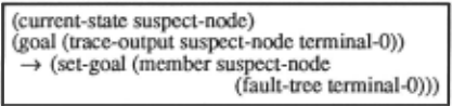
The use of the perceptual information is represented by the production shown in figure 6. This production replaces the trace-output by a fault-tree of the terminal 0 output and the suspect node is checked to see if it is a member of this tree. This can be generalized to generate the fault-trees of all the terminal Os, and then find the set of nodes common to all these trees at each level.

Hence we infer that the visual cue provides a pointer which indicates that the problem can be solved by tracing back the fault-tree from all the Os simultaneously. But the new strategy could not have evolved without the realization that at each level, the suspects are found by finding the intersection of all the set of suspects for each terminal 0.

5.3 Knowledge from Simultaneous Propagation

Since all the terminal 0 outputs are propagated backward to generate a fault-tree, a natural extension is to propagate back from terminal 1 outputs. Since all inputs to such com­ ponents have to be 1, all the components on the tree generated by back-propagating a terminal 1 output have to be functioning properly. Hence at each level, the subject eliminates all the components on the suspect-lists which also lie on the functioning-tree. This makes the search more efficient in terms of computations. This learning process can be implemented by providing adaptive productions which remove all the nodes, on the trees generated from terminal 1 outputs, from suspect lists.

5.4 Chunking

The use of chunking3 is clearly illustrated in problems P8 and P13. The subject has stored in long-term memory the information that the node that ultimately explains all ter­ minal 0 outputs is 17. This information was gathered in PS and stored in long-term memory. It was later recalled in P8 and P13 where all the terminal nodes have 0 outputs, and used effectively to reduce search. But this piece of chunked information was insufficient as there is another component (18) which can also results in a 0 at all terminal nodes. This caused the subject some trouble in PIS, when the faulty component was 18. Any search path that provides a set of root nodes that explain all the terminal 0 outputs is remem­ bered for future use. For example the fact that 17, 18 are two nodes that can explain all terminal Os is. remembered and used later.

In our experiments this is the only example of chunking that is apparent. The case mentioned above is remembered since it is related to the unusual set of all 0 outputs. It is expected that with increased practice, other symptoms would be chunked to their faulty component set and remem­ bered. In general, for any symptom one can generate the set of faulty components which explain all the outputs and this information can be chunked and stored in long-term memory.

5.5 Computer Simulation

Based on the analysis of protocols presented in the previous sections, we have implemented a production system which simulates the learning process. The production system, im­ plemented in OPSS, incorporates the four strategies used by the subject in successive problems. Each of the strategies are implemented independently and are executable indepen­ dently as well. In addition, we have implemented the learn­ ing process in terms of the four "learning operators" described in this section. These operators are implemented as productions which gather additional pieces of infor­ mation to evolve a better strategy with respect to the current strategy. For example, in the evolution of the refmed depth­ first from depth-first strategy(described in section 5.1), the information on the number of measurements required by the two characterizations of a faulty component is used in the reordering of the productions. This reordering results in reducing the number of measurements required for diag­ nosis. The implemented system simulates the strategy shifts from depth first to refined simultaneous-propagation strategy. The system, in simulating the strategy shifts, uses the same information as used by the subject but does not account for the temporal course of the subject's learning. The simulation ensures that the operators identified are suf­ ficient to explain the learning process.

6 Discussion

The subject has available in long term memory some general problem solving strategies. This supported by the fact that he is able to solve the first problem successfully as soon as it is posed by using the depth first strategy. The depth first strategy can be roughly approximated as meansends analysis [Newell and Simon, 1972]4. Although this strategy leads to the correct solution it is not optimal in terms of the problem objective of minimizing the number of measurements for a diagnosis. However, the computational requirements of the depth-first strategy are small. As the subject moves from the depth-first strategy to simultaneous propagation strategy, he is able to decrease the number of measurements to a diagnosis. However, the computational requirements of the corresponding strategies increase. We illustrate this by an example.

3Chunking has been proposed as a learning mechanism which records goal-based experience [Laird, Rosenbloom and Newell, 1984].

Consider the network in figure 1 with the following symptom: (1, 0, 0, 0, 0, 0, 0). Each digit in the vector corresponds to the output of the terminal node, from top to bottom. The faulty component is 20. The depth-first strategy requires 11 measurements, refined depth-first re­ quires 6, simultaneous propagation and it's refmed version require 5 (which is a minimum). Hence the diagnostic ef­ ficiency improves as we move from depth-first to simul­ taneous propagation. On the other hand, the computational load increases. In order to characterize the computational requirements of various strategies, we defme the number of rows as n and the number of columns as d in figure 1. The computational complexity of the depth first and its refmed version is of O(nxd), and that of simultaneous propagation is of O(n2xd).

The observation leads us propose that learning of new strategies is driven by competing objectives. The problem objective guides the subject to evolve strategies which min­ imize the number of measurements. The learning operators which transform the depth-first strategy to it's refined ver­ sion and subsequently to the simultaneous propagation strategy fall into this category. As the strategies that min­ imize the number of measurements impose larger computa­ tional requirements, the subject devises ways of alleviating these requirements in order to reduce the cognitive load. For example, the shift from simultaneous propagation to it's refined version does not improve the the number of measurements but reduces the computational effort. At each step, the refined simultaneous propagation strategy prunes all the components on the suspect list which have outputs to a I. This reduces the number of hypotheses that need to be considered at each step. Moreover, the number of hypothesis generated in the next step is also reduced. Chunking is yet another learning operator that provides a means to improve problem solving by utilizing previously recorded goal-based experiences. From our observation of the protocols, we think chunking also provides a means to generate structural abstractions on the device network.

In conclusion, this experiment has pointed out to us that the learning process is shaped by the interaction between the cognitive load and the problem objectives. Further, each dimension has its own set of learning operators.

7 Further Remarks

This work is proposed as a first step towards identifying computational mechanisms which can explain the genera­ tion of expertise from fundamental knowledge. Fundamen­ tal knowledge is concerned with ·_the first principles of the domain and is described in terms of a model of a device. Typically, novices in an area start out with this kind of knowledge. On the other hand, expertise consists of knowledge gained through experience. It provides "short cuts" through the knowledge which enables experts to solve the problems faster and more efficiently. The experiential knowledge consists of productions or rules which encode knowledge compiled from the first principles. This question is of special interest in machine diagnosis, where much research is directed towards integrating the use of model based systems with expert rule based systems.

Design of tutoring systems concentrate on the identifica­ tion of student models as means to develop didactic strategies. A variety of techniques for characterizing stu­ dent models have been proposed in the literature [Wenger, 1987]. In this study, we have explored the process of trans­ formation of a novice to an expert. This process is charac­ terizable in terms of information that the novice uses to evolve better strategies. This model of evolution could provide a basis for intervention to improve novice strategies for solving problems in a tutoring context.

Acknowledgements

We thank the reviewers for their comments.