
Towards Finding Optimal Solutions with Non-Admissible Heuristics: A New Technique
Proceedings of the Eleventh International Joint Conference on Artificial Intelligence. Search. Pages 303-307.
Abstract
A problem with A* is that it fails to guarantee optimal solutions when its heuristic, h, overestimates. Since optimal solutions are often desired and an underestimating h is not always available, we seek to remedy this. From a nonadmissible h an admissible one is generated using h 's statistical properties. The new heuristic, hm, is obtained by inverting h with respect to its own least upper bound function. The set of nodes expanded when A* uses g + hm as an evaluator is compared with the set of nodes expanded using other approaches which have been suggested in the literature. A considerable potential savings in node expansion when using hm is indicated. In 8-puzzle experiments A* using g +hm expands one fifth as many nodes as does the best alternative approach.
- [Bagchi and Mahanti, 1983] A. Bagchi and A. Mahanti, Search algorithms under different kinds of heuristics -A comparative study, JACM, 30(1):1-21, 1983.
- [Bagchi and Mahanti, 1985] A. Bagchi and A. Mahanti, Three approaches to heuristic search in networks, JACM, 32(1):1-27, 1985.
- [Chakrabarti et al., 1988] P. Chakrabarti, S. Chose, and S. C. DeSarkar, Admissibility of AO* when heuristics overestimate,Artificial Intelligence 34:97- 113, 1988.
- [Dechter and Pearl, 1985] R. Dechter and J. Pearl, Generalized best-first strategy and the optimality of A*, JACM, 32(3):505-536, 1985.
- [Gashnig, 1979] J. G. Gaschnig, Performance Measure- ment and Analysis of Certain Search Algorithms, Ph.D Thesis, Carnegie-Mellon University, 1979.
- [Huyn et al., 1980] N. Huyn, R. Dechter and J. Pearl, Probabilistic analysis of complexity of A*, Artificial Intelligence 15:241-254, 1980.
- [Korf, 1985] R. E. Korf, Depth-first iterative deepening: an optimal admissible tree search, Artificial Intelligence, 25:97-109, 1985.
- [Nilsson, 1980] N. J. Nilsson, Principle of Artificial Intelligence, Tioga Publishing Co., Palo Alto, Ca., 1980.
- [Pearl, 1984] J. Pearl, Heuristics, Addison-Wesley, Reading, Mass., 1984.
- [Politowski, 1986] G. Politowski, On the Construction of Heuristic Functions, Ph.D. Thesis, University of California, Santa Barbara, 1986.
References were extracted automatically from the PDF and may contain errors.
Full text extracted automatically from the PDF; figures, tables and equations may differ. The PDF is the version of record.
1. Introduction
A problem with A* is that it fails to guarantee optimal solutions when its heuristic, h, overestimates. Since optimal solutions are often desired and an underestimating h is not always available, we seek to remedy this.
Two approaches to this problem have been suggested in the literature. In one [Chakrabarti et al., 1988; Pearl, 1984 (p. 205)] an upper bound p on the worst case overestimation of h is obtained; ie, p = max{h(n)/h*(n): h*(n) > 0}, where h* returns the optimal distance to goal. Now set hp = h/p so that hp underestimates h*. A* with evaluator g + hp (denoted A *(hp ) is admissible. A problem with this is that when p is large, hp is weak; in the extreme case hp returns values less than the minimum edge length of the state space graph and its effect is only to break ties in a breadth-first search. The other approach is a two phase variation of Bagchi and Mahanti's C-algorithm [1983, 1985]. It requires additional information, such as p, above, and is called here C'(p). It is described in Appendix B.
The new approach described here uses a statistical sampling to learn more precise information about h 's overestimation. Namely, one estimates the maximum possible value of h(n) as a function of n 's true distance from goal. We denote this statistically learned function by maxh:
maxh(x) =max{ h(n): h*(n) = x }, x ~ 0.
If p may be obtained from samplings, then the same measurements taken may be used to estimate maxh. If p can be obtained from domain specific theoretical considerations, then these same considerations might enable the upper bound to be a function of distance to goal, ie, they may be used to ascertain maxh. From han underestimating heuristic hm is built using maxh by defining
hm(n) = min{x: h(n) ~ maxh(x)}
for all nodes n. The heuristic hm is no less informed than hp in the sense that hp ~ hm ~ h*. If we had hp < hm on all non-goal nodes, then we could conclude that all nodes expanded by A *(hm) are expanded by A*(hp) [Nilsson, 1980]. Unfortunately the inequality is not strict. A simplified search model, due to Huyn, Pearl and Dechter [Huyn et al., 1980], when applied to this situation, implies that the non-strict inequality is adequate to assure that the expected number of nodes expanded by A *(hp) is greater than or equal to the expected number expanded by A*(hm>· However, we would like a more detailed statement of which nodes may be expanded by A *(hp), A *(hm) in order to better compare the two algorithms with each other and with C'(p).
In sections 4, 5 we described the nodes expanded by A*(hp), A*(hm) and C'(p) by specifying lower and upper bounds for them, ie sets of nodes which are surely expanded (SE) and possibly expanded (PE) by each algorithm. These SE and PE sets are defined in terms of whether or not certain "constrained" paths have their nodes expanded. The path constraint for each of the three algorithms is expressed in terms of the original non-admissible heuristic h; this allows a direct comparison of the three node-expansion sets. The paths explored by the three algorithms are plotted on a single graph. It is seen that, when maxh is non-linear, the potential savings in node expansion when using A *(hm) instead of A *(hp) is considerable. It increases as distance between start and goal increases. C'(p) is seen to be substantially slower than the other two algorithms. We also show how SE and PE set containment may be used in a direct way to rank the speed of the algorithms.
All three algorithms were run on the 8-puzzle using the enhanced Manhattan distance for an overestimating heuristic. On average A *(hp) expanded 5 times as many nodes as did A *(hm). As problem difficulty increased the comparative behavior of A *(hm) improved. As expected, C'(p) ran considerably slower than A *(hp). Details are in section 6. Section 7 discusses methods for building hm and section 8 concludes.
2. Notation
| s | start node |
| g*(n) | length of cheapest path from s ton |
| h*(n) | length of cheapest path from n to a goal |
| g(n) | length of cheapest path found so far from s to n by a search algorithm; also length along a particular specified path in section 4 |
| h(n) | estimate of h*(n); assume h(goal) = 0 |
| C* p | h *(s) · max( h(n)/h*(n): h*(n) > 0 ) |
| hp maxh(x) | h/p max( h(n): h*(n) = x) |
| hm(n) | min( x: h( n) ~ maxh( x) ) |
| A *(h) | A* algorithm using g + h as evaluation function |
The state space graph is assumed to be a locally finite directed graph with arc length bounded below by a positive number. We assume a solution path exists. A heuristic function h is called admissible (=underestimating) if h ~ h*.
3. Basic Properties of hm
Let h be a non-admissible heuristic function. In order to build an admissible function from it we first obtain maxh:
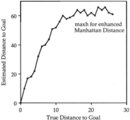
This may be learned by doing a statistical sample of the values returned by h on nodes a known distance from the goal. For example, Figure 1. shows maxh when h is the enhanced Manhattan distance in the 8puzzle. The latter is simply the Manhattan distance plus a rotational term see Nilsson [1980]. The data were gathered by Gaschnig. (See Gaschnig [1979] where the sampling techniques and confidence levels are discussed.)
Define hm on nodes n via
Since h(n) ~ maxh(h*(n)), one of the x-values on the right side of (2.1) is h*(n). Thus hm(n) ~ h*(n) so hm is admissible. hm is no less informed than hp in the sense that hp ~ hm. To see this, notice that maxh(x) ~ px and that the right side of (2.1) defines hp when maxh(x) is replaced by px.
Let MAXH(x) = max(maxh(t): t ~ x) so that MAXH is like maxh except that when maxh values decrease those of MAXH remain constant; ie, MAXH is non-decreasing. If maxh is replaced by MAXH in (2.1), the values of hm are unchanged. Hence we may assume, without loss of generality, that maxh is non decreasing and defined for all x E [O,C*]. This is done in the sequel.
4. Nodes Expanded: C'(p), A *(hp), A *(hm)
Let P be a path emanating from the start node. Let R be some constraint on the nodes of P. For example, R might be the requirement that nodes n satisfy g( n) ~ C*, where g is understood to mean distance from start along P and C* denotes optimal distance from start to goall . We say Pis R-constrained if every node on P satisfies R. The set of all nodes n such that there is an R-constrained path connecting s to n is denoted S[R]. For any search algorithm A let E(A) denote the nodes expanded by A. The following theorem (proof in appendix) gives upper and lower bounds for the set of nodes expanded by A *(hp), A*(hm) and C'(p). In the theorem, a comma within a constraint specification denotes logical AND.
1. As used here, g is a function of P and n. The more precise symbol, used in the appendix, is C(P,n) instead of g(n).
Theorem 4.1: Assume that h is non-admissible. Then
where in (a) it is the case that Q ~ C*.
Let A be any of the three algorithms above. We call the left sides of (a), (b), (c) the nodes possibly expanded by A, symbolized PE(A), and the right sides the surely expanded nodes, symbolized SE(A). (The latter term has been used in [Dechter and Pearl 1985].)
The nodes expanded by the three algorithms may be represented as planar regions. As an example we take maxh to be a smoothed version of that obtained by Gaschnig in Figure 1. From Gaschnig's data we calculate p = 10. In Figure 2 the x-axis. represents g values assumed at nodes n on paths emanating from start. They-axis represents the corresponding g(n) + h(n) value. A particular node n may have several 'coordinates', (g(n), g(n) + h(n)), in this scheme, depending on which path from s to it is considered. Curve eb represents the points (x, x + maxh(C*- x)), where 0 ~ x ~ C*. Applying the theorem to Figure 2 shows that PE(A*(hp)) and PE(A*(hm)) are represented, respectively, by nodes lying on paths from start which stay within abd and abe. The same is true for SE(A*(hp)) and SE(A*(hm)), except that now, essentially, the paths are not allowed to touch bd and be, respectively. Figure 2 shows that the saving in node expansion by using hm rather than hp is potentially very large when maxh is non-linear. Furthermore, it increases as C* increases.
The theorem also shows that SE(C'(p)) consists of the nodes on paths within abed' along with paths within aqf. This area is substantially larger than that for PE( A *(hp) and PE( A *(hm)), indicating a relatively slow algorithm.
5. Ranking the Algorithms
In comparing the speeds of two algorithms A and B, one would like to show that E(B) ::::J E(A) (or vice pQ] d'
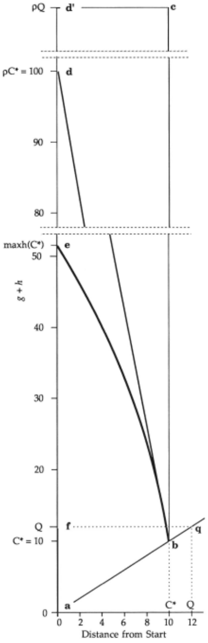
versa). One then says that A dominates B. Proving dominance for large classes of problems is difficult and not always achievable. However, in theorem 4.1 the upper and lower bounds placed on E(A) by PE(A) and SE(A) differ only by an'=' or an 'e within a path constraint. This considerably restricts possible values for E(A). Therefore we propose using PE and SE set containment to get an approximate idea of which of several competing algorithms is fastest. Algorithm A is said to have bounded dominance over B, written A> B, if we always have SE(B) .::::J SE(A) and PE(B) .::::J PE(A). By the theorem, A*(hm) > A*(hp) > C'(p). Accordingly, we expect A *(hm) to expand the least number of nodes and C'(p) the most.
6. Experimental Data
All three algorithms were run on the 8-puzzle using the enhanced Manhattan distance for an overestimating heuristic. Gaschnig's statistics (Figure 1 and [Gashnig, 1979]) were used for p and maxh. Accordingly, p was set to 10. Table 1 shows comparative data for nodes expanded by A*(hp) and A *(hm>· In this sample there were 222 problems with start-goal distances between 3 and 21. On average A *(hp) expanded 5 times as many nodes as did A *(hm). As problem difficulty increased, the comparative behavior of A *(hm) improved. For example, when start-to-goal distances were 21, A *(hp) expanded 6 times as many nodes as did A*(hm) while, for start-goal distances of 17, the ratio was 4. These distances can be as large as 29 in the 8-puzzle and the most frequent distance is 24. However, we ceased sampling when A*(hp) required more than one day per problem on our facility (IBM 3083).
C'(p) ran considerably slower than A *(hp) so statistics were not collected for it. Both A *(hp), A *(hm) returned only optimal solutions in this sample. However, since hp, hm are built from statistically gathered data, this need not always happen.
| D | No. of | nodes expanded (avg.) | Ratio | |
|---|---|---|---|---|
| problems | A*(he.) | A*(hm) | ||
| 21 | 21 | 10377 | 1766 | 5.88 |
| 20 | 59 | 6213 | 1261 | 4.93 |
| 19 | 48 | 4330 | 875 | 4.95 |
| 18 | 28 | 2588 | 586 | 4.42 |
| 17 | 27 | 1797 | 450 | 3.99 |
| 3-16 | 39 | 579 | 168 | 3.45 |
| 3-21 | 222 | 4216 | 849 | 4.96 |
7. Building hp, hm
The techniques described in this paper all require information about the behavior of the non-admissible heuristic h.
A*(hp) and C'(p) require p and A*(hm) requires maxh. The problem of how to obtain such information has never been addressed: Chakrabarti [1988] says that 'if the proportional error H/H* is bounded above bye, then .. .'; Bagchi [1983] says 'suppose Qopt ~ aQ for some given constant a > 1, .. .'; and Pearl [1984] writes: 'when a heuristic h, is known to overestimate h* cosistently, ... then the use of h2 = ah, with a < 1 may be justified .. .' However no-one has suggested how to obtain the critically needed constants (e, a or p). In some cases theoretical insight about a problem domain may reveal p, maxh. The only general methods of which we are aware involve statistical sampling. In this case p, maxh are known with imperfect confidence.
To estimate p, maxh one needs to sample a large number of h(n)-values for each of many possible h*(n)-values. Even when· the h*(n)-values are known with certainty, the critical nodes n may not have been examined, consequently the estimates of p, maxh may be too low. The corresponding heuristics, may overestimate. Confidence in their admissibility increases with confidence in the estimates of p, maxh.
There are several possible approaches, some of which we mention below.
(1) A breadth-first expansion of the state space from several possible goals provides good information, but only for small h*(n)-values due to likely combinatorial explosion. However such limited data may suggest that maxh is essentially concave down (as in Figure 1), causing p to occur early. (It occurs at h*(n) = 1 in Figure 1.) To the extent that this is believed, one may wish to build hp from such limited data.
(2} If a weak admissible heuristic is known, then it may be used with A* to find optimal paths between randomly generated start-goal pairs. From these paths, desired statistics may be obtaiained . IDA* [Korf, 1985] rather than A* could be used. The problem here is that a weak heuristic may not enable the discovery of long optimal paths within reasonable computer resources. (This method raises another question: will the 'admissibilized' heuristic expand fewer nodes on average than the admissible heuristic used to generate the statistics? In the 8puzzle we have created hm 's stronger than tiles-out of place (a weak admissible heuristic), but not stronger than the Manhattan distance. Had the former been used to generate our statistics, then the answer would be 'yes'. Other domains need to be studied.)
(3) Goals are selected randomly from the state space. Random walks are made from each of these goals into the state space; from the nodes reached, data are collected regarding maximum h-values corresponding to apparent h""-values (as measured along the walk). The result is an even lower estimate of p or maxh than would be the case if accurate h""-values were known2. However, one can build up confidence in such estimates by taking a sufficiently large sample. This method has been suggested in a different context by Politowski [1986].
A combination of the above methods may be used to build better and better estimates of maxh. If a domain is to be repeatedly searched, then this searching may itself be combined with learning better estimates of maxh.
The problem requires further study. Another interesting problem is that of relating statistical confidence in the estimate of maxh -to statistical confidence in the admissibility of A ""(hm).
8. Conclusions
We have shown that an overestimating heuristic h may be made admissible by using a statistically learned non-linear transformation. When used with A"", the new heuristic enables optimal goals to be found while expanding fewer nodes than does any previously suggested technique which is also based on h.
All previous methods use some additional information about h 's behavior, namely p. The method described here uses more detailed information, namely maxh; but the same measurements taken to statistically estimate p may be used to estimate maxh. The initial estimation cost may pay off if A"" is to be run repeatedly in the same domain and an acceptable admissible heuristic is not available. In all these methods confidence in admissibility is based on confidence in the statistical estimates of p or maxh.
Appendix A. Notation for Appendices B, C
- Open nodes which are candidates for expansion in A"" and similar algorithms
- C(P,n) length of path P from s ton
- M(P) max{C(P,n) + h(n): n is on P} where Pis some solution path
- Q min{M(P): P is a solution path}, called the first discriminant
Qopt min{M(P): P is an optimal solution path}, called the second discriminant
The last four terms are from [Bagchi,1983].
2. To see this recall from section 3 that maxh = MAXH.
Appendix B. A two-phase admissible search algorithm
Bagchi and Mahanti [1983] describe an algorithm, C, which yelds high solution quality and reexpands fewer nodes than A"". They point out that a 2-phase variation, which we call C'(p), may be used to find optimal solutions when heuristics overestimate.
The essential control part of C'(p), is shown in Figure 3. We use the symbol Open(t) to denote {n: n E Open, /(n) ~ t } and call this the focus; t is called the focus bound. F in line 3.1, 3.3 is the largest value yet of min{ f(n): n E Open }. In phase 1 C is run to completion obtaining a possibly non-optimal goal, say n. This phase ends when the test at line 3.5 is positive. At this point the value of F is Q, the first discriminant. The whole point of phase 1 is to find Q.
In the second phase an upper bound for Qopt/Q is required. p works (Lemma C1, in Appendix C) In lines 3.6, 3.7 n is returned to Open and the focus bound is set larger than Qopt (namely pQ ), where it remains for the duration of the search. Focused nodes and their focused descendants are now breadth-first expanded until a (second) goal is found. This goal will be optimal because the focus bound is large enough to assure that nodes on some optimal path can be 'focused', and a breadth-first selection finds this solution path first. If n was optimal, then it will be rediscovered, but now with knowledge of its optimality. The idea of the algorithm is that presumably breadth-first expanding only nodes which qualify for focus and have g-values less than g( n) is faster than conducting a blind breadth-first search from start considering all of Open.
- Insert(s, Open), F <-- 0
- Repeat until Open is empty or n is the second goal
- If Open(F) = tP then
- F <-- min{ /(m): m E Open }
- n <-- a node on Open(F) with the smallest gvalue;
break ties in favor of a goal node.
- If n is the first goal then
- F <-- p F
- return n to Open
- If n is not a goal then expand n ...
Figure 3. A two-phase algorithm for finding optimal solutions when h overestimates (reworded from [Bagchi and Mahanti 1983]).
Appendix C. Proofs.
LemmaCl
(1) C"" ~Q ~Qopt
- Q0pt ~ pC* ~ pQ, where h is non-admissible
- If his admissible, then C"" = Q = Qopt
Proof
- (l):Take P0 such that Q = M(P0 ). Then C* ~ length(P0 ) ~ M(P0 ), proving the left side. The right side is obvious.
- (2):Qopt = min{max{C(P,n) + h(n): n is on P): Pis an optimal solution path) ~ max{C(P,n) + ph""(n): n is on P, P is an optimal solution path) =pC*,
proving the left side. The right side follows from this and (1).
- (3): If h is admissible, then the previous argument shows (2) with p= 1. (3) now follows from (1) and (2). A
TheoremCl
S[g + h ~Ql ~ E(A*(h)) ~ S[g + h < Ql
Proof See [Bagchi and Mahanti, 1985]. A
Proof of Theorem 4.1
- (a) Consider the left containment. The S[g + h ~ QJ term comes from the first phase of C'(p) and follows from the definition of Q. (See [Bagchi and Mahanti, 1985] for more discussion.) In the second phase we expand in a breadth-first fashion all nodes q reachable from s by an R constrained path P where R forces C(P, q) + h(q) ~ pQ. Since an optimal goal will be found in this fashion, all nodes q so expanded satisfy C(P, q) < C*. This proves the first half of (a). The proof for the second half is similar.
- (b) By Lemma C1 and Theorem C1, S[g + hp ~ C*] ~ E(A *(hp)) ~ S[g + hp < C*J. Since h = php, the assertion follows.
- (c) Assume n E E(A*(hm)). By Lemma C1 and Theorem C1, n is on a path P from s to n whose nodes q satisfy g(q) < C* and hm(q) ~ C* - g(q), where g(q) is an abbreviation for C(P, q). By definition of hm, we have for each q on P that there exists some xq such that xq = hm(q) ~ C* - g(q) and h(q) ~ maxh(xq). Applying maxh to the first relation and using the second gives h(q) ~ maxh(C*- g(q)), because we may suppose maxh is non-decreasing. Since this is true for every q on P, the first containment of (c) is shown.
For the second containment, take arbitrary e > 0 and let P be a path from s whose nodes q satisfy the required constraints. For such q, h(q) ~ maxh(C*- C(P, q) -e), and hence the least x such that h(q) ~ maxh(x) must be ~ C* - C(P, q) - e. Thus hm(q) < C*- C(P, q) for nodes on P. It follows that the right side of (c) is contained in S[g + hm < C*J which is itself contained in E( A *(hm)) by Theorem C1 and Lemma Cl. A
The authors wish to thank Professors Richard Korf, Jack Mostow and the referees of this paper for helpful comments and suggestions.
@inproceedings{ijcai1989p48,
  title     = {Towards Finding Optimal Solutions with Non-Admissible Heuristics: A New Technique},
  author    = {Davis, Henry W. and Bramanti-Gregor, Anna and Chen, Xiaoteng},
  booktitle = {Proceedings of the Eleventh International Joint Conference on
               Artificial Intelligence, {IJCAI-89}},
  publisher = {International Joint Conferences on Artificial Intelligence},
  editor    = {N. S. Sridharan},
  pages     = {303--307},
  year      = {1989},
  month     = {8},
  note      = {Search},
  url       = {https://ijcai.org/proceedings/1989/48},
}
TY - CPAPER TI - Towards Finding Optimal Solutions with Non-Admissible Heuristics: A New Technique AU - Davis, Henry W. AU - Bramanti-Gregor, Anna AU - Chen, Xiaoteng T2 - Proceedings of the Eleventh International Joint Conference on Artificial Intelligence, IJCAI-89 PB - International Joint Conferences on Artificial Intelligence PY - 1989 SP - 303 EP - 307 UR - https://ijcai.org/proceedings/1989/48 ER -Copied
Machine-readable versions of this paper, for tools and AI agents:





