Rapid Retrieval Algorithms for Case-Based Reasoning

1 Introduction

1.1 Problem Statement

Rapid development of expert systems is hindered by the well-known knowledge acquisition bottleneck. Case-Based Reasoning (CBR) overcomes this problem by representing knowledge as cases, where each case consists of a problem and its solution. A problem can be solved by remembering the solution to a similar problem and adjusting it for the current context [Kolodner et al., 1985]. If a case base contains enough cases, these adjustments can be very simple. However, retrieving the most similar cases from a very large case base can be time-consuming. Our research has focused on developing efficient algorithms for case-based retrieval.

The fundamental principle of case-based reasoning is that problems are solved based on a memory of a prior similar situation. A similar situation is acquired through reminding of an individual event or an abstraction through long term memory associations (episodes) [Kolodner and Riesbeck, 1986, Schank, 1982].

Many issues are raised when discussing reminding, or retrieval, of prior episodes in a CBR system [Owens, 1988]. CBR system developers have many responsibilities related to James A. King NCR Corporation 1700 South Patterson Boulevard Dayt()n, OH 45479

*This reseaich was supported in part by the Defense Advanced Research Projects Agency under contract number DAAH01-88C-0341, and in part by the Air Force Weapons Laboratory under contract number F33-61 5-87 -C-5300.

creation of the case-base and the supporting retrieval functions. A developer must understand the breadth of knowledge which must be provided in each case, including case-specific attribute knowledge and general, or domain-specific, knowledge. A developer must understand the definition, and application of, the sim~larity-metric for the domain. A similarity-metric is the measunng scheme used to describe how a combination of new situ_ation's attribute values correspond to a prior case, or case's, attnbute values. A developer must understand what forms of retrieval can be utilized in the reminding process of the CBR system, and what scheme should be used for indexing or classification. In this paper we respond specifically to the problem of providing efficient retrieval algorithms for case-base reminding.

We have identified three types of retrieval, quantitative retrieval, qualitative retrieval, and a combination of the two. In quantitative retrieval (specifically directed at domains containing numeric representations of information), the values of a c~e's attributes are numeric and the similarity between any two cases is defined as the inverse of the distance between them. If two cases are similar, the distance between them is small. As the difference between their attribute values increases, their distance increases.

In qualitative retrieval, a case's attributes are qualitative values, such as colors or names. Similarity is defined as the number of exact matches between attribute values, perhaps employing a weighting scheme to emphasize the importance of a particular attribute. It is important to note that in this situation it is generally not possible to simply perform a search using the most important attribute first. The closest case may ~ot match on the most important attributes but on many less Important ones, especially if the weights are similar for all attributes.

Combined quantitative and qualitative retrieval is necessary for cases which have both quantitative and qualitative attributes.

1.2 Problem Solution

The algorithm developed for quantitative retrieval makes use of a graphical paradigm. Cases are represented as points in a hypersp_ace, where the dimensions of the space correspond to ~he attnbutes of the case. The space is recursively divided mto hypercubes (squares for two dimensions, cubes for three, etc.). Each cube contains zero or more points up to a small number. Retrie~al of the closest point to a point of interest is reduced to finding the hypercube that would contain the point of interest.

The qualitative retrieval algorithm uses a tree and hashing scheme to efficiently test every possible combination of attributes to determine exact matches. The combined retrieval algorithm is a simple combination of these two algorithms.

1.3 Related Work

Case-Based Reasoning can only be productive to a user if prior experiences can be retrieved efficiently to use in the retrieval process [Martin, 1988]. Martin goes on to state that the CBR system must continue to perform at an efficient level of retrieval while the case-base grows considerably. CORA is described as a system that stores cases in an overlapping fashion which allows for reconstruction. This is in contrast to the general method of storing cases as individual portions of memory. Our paper provides a view of retrieval on individualized cases and feature sets.

[Owens, 1988] presents the problem that case memory is not static and does not enjoy advanced ordering of features. In particular, CBR systems do not always have a static understanding of the measure of similarity. The similarity metric will change over time and growth of the case-base. Owens concluded that discrimination trees provide adequate support if the case-base is static.

[Preparata and Shamos, 1985] describe a well-known computational geometry algorithm for retrieving from a set of existing points, the closest point to an arbitrary point. This algorithm is based on the Voronoi diagram which divides the space into volumes, one volume for each point. Finding the closest point reduces to finding the volume which the arbitrary point falls into. This can be done in O(Log(N)) time, where N is the number of points. Unfortunately, the amount of space required to store the volumes is impracticably large except in the two dimensional case. However, this retrieval algorithm was the starting point for the development of our quantitative retrieval algorithm.

[Corkill et al., 1986] classify the dimensions which define a blackboard space into ordered and enumerated. Their ordered dimensions correspond exactly to our quantitative dimensions. Their enumerated dimensions correspond with our qualitative dimensions except that our qualitative dimensions allow an infinite number of values while theirs assume a finite set. They also discuss retrieval based on dimensions with concern for efficiency of the operations.

[Samat, 1988] discusses uses of quadtrees especially as they relate to storage and retrieval of rectangles. Our qualitative retrieval algorithm is based on a quadtree representation.

1.4 Paper Organization

Section 2 describes the three retrieval algorithms in detail. Section 3 presents an analysis of the algorithms. Section 4 provides empirical results and Section 5 suggests directions for future research.

2 Description of the Retrieval Algorithms

2.1 Voronoi-Inspired Quantitative Retrieval Algorithm

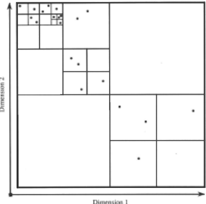
The graphical nature of the Voronoi retrieval algorithm prompted us to search for a graphical retrieval algorithm practical for more than two dimensions. The resulting algorithm is termed the Voronoi-Inspired (VI) Quantitative Retrieval algorithm. The VI algorithm performs a preprocessing step, in which a hypercube containing all the data points or cases is recursively divided into smaller hypercubes until no hypercube contains more than a certain number, m, of points. Note that this means that a hypercube may be empty, but one of its neighbors must be nonempty. Figure 1 shows an example of hypercube sub-division where the maximum number of points per cube is two (this value would be unrealistically low from an efficiency standpoint). The retrieval of the closest point (most similar case) consists first of fmding the hypercube that contains the test point.

Dimension 1

Figure I Hypercube Subdivisions

Then, points in that hypercube and, in some circumstances, bordering cubes must be examined for proximity.

The integrity of the algorithm depends on the definition of distance between points. The distance formulation should treat all dimensions monotonically, symmetrically and identically. The distance between points depends on the differences between their attribute values. Treating dimensions monotonically means that as these differences increase, the distance increases. The magnitude of the increase cannot depend on the sign of the difference or on the dimension. Both the geometric definition of distance (square root of the sum of the squares) and the sum of the absolute values of the differences satisfy these criteria.

In many applications, a weighted sum will be necessary in a definition for distance. However, a weighted sum does not treat all dimensions identically. In order for the VI algorithm to be applicable, all the weights must be equal. This is handled by simply multiplying all the attribute values of a point by their weights before the point space is preprocessed into smaller and smaller hypercubes.

In one of our applications, SUR VER III [King et al., 1988], it was clear that differences were not as important as multiplicative factors. For example, a case with a peak blast overpressure of 1 Mpa was closer to a case with a peak blast overpressure of 3 Mpa than to a case with 0.1 Mpa. The differences are 2 Mpa and 0.9 MPa respectively, but the multiplicative factors are 3 and 10. Therefore, SURVER III defined distance as the weighted sum of the. multiplicative factors. The multiplicative factors are not symmetric (distance increases faster as a dimension goes toward 0) so the VI algorithm was not directly applicable. However, by taking the log of the dimension before the preprocessing step (and multiplying by the weights), we were able to achieve the desired results.

2.2 Tree-Hash Qualitative Retrieval Algorithm

The Tr~e-Hash Qualitative Retrieval algorithm was designed for retneval of cases whose attributes have qualitative values. Retrieval of a qualitative case is very efficient if we know a priori which dimensions or attributes of the current case will match attributes of cases in the case base. However, this information is never available ahead of time. The Tree-Hash algorithm overcomes this problem by maintaining multiple pointers to cases - one for each possible combination of the dimensions. For example, in the two dimensional case with dimensions d1 and d2, the possible dimension combinations are {d1, d2, d1d2}. The algorithm attempts a retrieval based on each of these combinations and computes a similarity measure. In our example, we first perform a retrieve based on d1, meaning that d1 is the only dimension that must produce an exact match. The same is done for d2. Retrieval based on d1d2 indicates that both dimensions must match the dimensions of a case in the case base. The algorithm is very fast when the number of dimensions is low. Retrieval time does not increase with the number of cases if a hashing scheme is used. Various versions of the algorithm are described in detail in the following sections.

2.2.1 Assumptions and Definitions

The Tree-Hash algorithm assumes that there are a large number of cases in the case base and a possibly infinite set of possible attribute values. The number of dimensions is relatively small and finite. Best match of dimensions is defined as the weighted number of matches of the qualitative values. In the case of ties for best match, any best match is acceptable. This requirement is necessary because the number of ties for best match can be an extremely large number of cases, especially if all dimensions are weighted equally. In the discussion below, the following definitions hold:

N = number of stored cases

D = number of retrieval dimensions

di = the ith dimension

2.2.2 Preprocessing

The Tree-Hash preprocessing step generates all possible combinations of attributes and represents them as nodes in a tree. The dimensions are placed in decreasing order of importance and labeled d1 through dD. The following algorithm generates the tree structure displayed in Figure 2, when the number of dimensions, D, equals four.

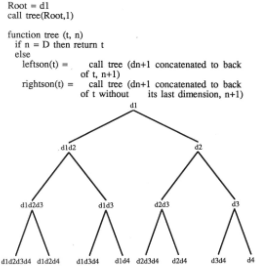
To provide efficient lookup, a unique pointer is created for each case and placed in a hash table exp(2,D) - 1 times, once for each possible combination of attributes, ignoring order. For each case, every node in the tree is visited. When a node is visited, the case is hashed using the dimensions represented by the node. The result of this process is a large hash table which encompasses all the cases, organized by every possible ordering of dimensions. Retrieval can now simply consist of visiting the nodes of the tree and performing a hash lookup based on the dimensions of the node.

2.2.3 Naive Retrieval

The simplest retrieval scheme involves traversal of the entire tree in search of a case most similar to the case of current interest. At every node, an attempt is made to retrieve a case and a record is kept of its measure of similarity to the current case. By comparing the similarity measures from the different nodes, the best match can be found.

2.2.4 Tree Traversal

Instead of visiting every node in the tree, it is more efficient to search the tree in a specified order to eliminate many of the hash retrievals. Traversal of the tree begins at the root. At each node, an attempt is made to hash retrieve a case based on the dimensions of that node. If the retrieval is successful, we proceed down the left branch. If unsuccessful, we proceed down the right branch. This process is continued until a leaf node is reached. At this point, we store the similarity measure from the node of the last successful retrieval. We then backtrack to the last successful node and follow its right son and proceed as before. This process is repeated until there are no successful nodes left to backtrack to. We then compare the stored similarity measures and select the best one. Using this scheme, a number of unpromising nodes never have to be visited.

2.2.5 Smart Tree Traversal

While the tree traversal algorithm given above avoids visiting some of the nodes of the tree, it can be improved. This is accomplished by computing and storing a score for each node of the tree during the preprocessing stage. The highest possible score at any node is the maximum of the possible scores of its subnodes. At a leaf, the score is computed, for instance, as the weighted sum of the number of dimensions. Tree traversal proceeds as in the previous algorithm, except that at each visited node, we compare the similarity measure of the retrieved case to the score at that node. If the similarity measure is equal to or better than the score at the current node, then the subtree under that node does not have to be traversed. This further reduces the number of nodes that have to be examined.

2.3 Combined Quantitative and Qualitative Retrieval Algorithm

To retrieve similar cases when the case base contains both qualitative and quantitative dimensions, we use an algorithm which is a straight-forward combination of the two previously described algorithms. The dimensions of the case must first be divided into qualitative and quantitative groups. A tree should be generated as described above using only the qualitative dimensions. At each node of the tree, we define pointers corresponding to each possible value of the qualitative dimensions at that node. For example, if the values of dimension d1 are {a, b} and the values of dimension d2 are { c, d}, we would define a set of pointers for the combinations { ac, ad, be, bd}. Each of the pointers is directed toward that segment of the case base which has matching dimension values. Each segment is then divided along its quantitative dimensions according to the VI algorithm.

To retrieve the most similar case, every node of the tree is visited. At each node, retrieval is first attempted based on the qualitative dimensions represented by the node. When a ~atching case exists for these dimensions, we perform a VI r~tnev3:l on the segment of the case base with corresponding dimensiOn values. We must also consider the situation where none of the qualitative dimensions match. A similarity score is computed for the node and retrieval proceeds to another node. The case with the highest similarity score is the closest match.

3 Analysis of the Retrieval Algorithms

3.1 Analysis of the VI Algorithm

3.1.1 Time and Space Requirements

A best case analysis of the VI algorithm indicates that the retrieval time can be expressed as:

K1 * Log (N/m) + K2 * m, where N = the number of cases, m = the maximum points allowed per atomic hypercube, Kl and K2 are constants

The first te~ is due to the search required to identify the proper atormc hypercube and the second term is due to a search through the points in that and nearby cubes. A probabilistic analysis using random cases shows that the mean retrieval time is the same expression as that for the best case but with larger constants. '

Th~ ~orst case re~eval time. can be made arbitrarily !arge. Th1s 1s done by usmg a very nght cluster of cases with JUS~ a f~w cases very far away so that the largest hypercube is arbttranly larger than the cluster containing most of the cases. By making this outer cube larger, more divisions are necessary to get a cube that immediately surrounds the cluster.

The time required to add a new case to the case base is proportional to the time to retrieve a similar case. The preprocessi.ng time, which consists of adding N points to the case-base, 1s O(N*Log(N/m)). The required space is O(N).

3.1.2 Advantages and Disadvantages

. The obvious advantage of the VI algorithm is that it 1s v~ry fast compared to other methods. It is also surprisingly appl~cable when combined with preprocessing steps which man~pu.late. the va!ues of the .cases' attributes through m~luphcatiO!l by wetghts, computation of logarithms, etc. The pnmary disadvantage of the algorithm is that it treats similarity identically throughout the case base. A change in the definition of similarity requires relatively slow preprocessing before rapid retrieval can again be performed.

3.2 Analysis of the Tree-Hash Algorithm

3.2.1 Time and Space Analysis

The Naive Retrieval strategy requires a hash retrieval at every node. There are exp(2,D) - 1 nodes in the tree and t~e hash retrieval takes constant time, resulting in a retrieval ume of K1 * (exp(2,D) - 1), where D is the number of dimensions and K1 is a constant.

For Tree Retrieval, the worst case retrieval time is still O(exp(2,D)), but the best case is O(D). Computation of the average retrieval time requires additional assumptions and a probabilistic analysis.

For Smart Tree Retrieval, the worst case retrieval time is still O(exp(2,D)). The best case retrieval time is a constant. The average retrieval time can be calculated from additional assumptions and probability theory.

To add a new case requires exp(2,D) - 1 hash inserts. Therefore, to preprocess all of the N cases (add a new case N times) requires time of O(N*exp(2,D)). The space required is also O(N*exp(2,D).

3.2.2 Advantages and Disadvantages

The biggest advantage of the Tree-Hash algorithm is its speed. The retrieval time does not increase as the number o~ cas~s increases. A change to the importance of the dimensiOns does not require extensive re-preprocessing as long as the same retrieval dimensions are used. Only the tree itself must be regenerated, which can be done very rapidly.

The Tree-Hash algorithm has a couple drawbacks. The retrieval time increases exponentially with the number of dimensions used for retrieval. For practical use of the algorithm, the number of dimensions is kept to about ten. The definition of similarity must be based on exact matches of the attribute values. This requirement limits the applicability of the algorithm. However, this can be partially overcome by defining new retrieval dimensions for the case base. For example, in a case base containing information about movies, we may have a dimension called "Country of Origin". While we recognize that movies from the United States, England and Australia are in some sense more similar to each other than to a movie from France, the similarity definition cannot capture this. We, therefore, add a new dimension called "Language Spoken" and now have a means of correlating movies in this manner. If new dimensions are added to the case base, the preprocessing step must be performed again.

3.3 Analysis of Combined Retrieval Algorithm

The worst case retrieval time for the combined retrieval algorithm is:

K1 * exp(2,D) * (K2 * Log(N/m) + K3 * m), where D = the number of qualitative dimensions, N = the number of cases, m is the maximum allowable points per hypercube, K1, K2 and K3 are constants

The first term results from searching through the tree and the second term results from performing the VI algorithm on the segment of the case base at each tree node. Note that in most circumstances the algorithm will perform much better than the W?rst case. because every segment pointed to from a tree node wlll contam only a small fraction of the cases.

4 Empirical Results

4.1 Quantitative Retrieval Empirical Results

A .uni~orm random number generator was used to generate pomts m a hypercu~e of two dimensions (a square box). 100, 1000, and 4000 pomts were used for three different sets of experiments. . A value of 2 was used for m (the maximum number o~ pomts allowed before a box was quartered). This was a de!t?erate attemp~ t? make the algorithm perform badly by explmtmg small vananons in the point distribution.

The minimum average depth of nesting for all atomic boxes is the log of N/m to the base 4. When m = 2, this produces 3, 5, 6, and 8 for N = 100, 1000, 4000, and 50,000

respectively. Our experiments suggest that the actual depth of an atomic box is very rarely greater than one more than this minimum number. The best case results hold within a constant factor. The retrieval time is fast enough to allow disk space to be used to store the indexing, thus keeping local memory from being a limitation. A random sampling of the boxes revealed that the boxes are only empty less than 25% of the time, despite the low value of m.

From the experiments, it is clear that the VI algorithm will work extremely well, when it is applicable. A question that remains to be answered through development of case based applications, is how often real data approximates random data and how limiting the restrictions placed on the distance definition are.

The VI algorithm has been successfully used in a practical instance of case based reasoning involving purely quantitative data. The algorithm was applied after a preprocessing step in which the logs of the attributes were taken and those results were multiplied by selected weights. One attribute of the problem that tended to make the VI algorithm applicable, was that the ultimate end users were novices and would not want to frequently redefine the similarity expression themselves.

4.2 Tree-Hash Algorithm Empirical Results

We are currently working on a manufacturing proposal case base consisting of fifty thousand cases. It appears at this early stage that the Tree-Hash algorithm is applicable. The number of retrieval dimensions is approximately six. Consequently, the exponential term in the retrieval time expression is not worrisome.

5 Future Directions

The three retrieval algorithms presented here are part of a DARPA sponsored case based reasoning shell currently under development. As part of the shell, these algorithms will compete with other retrieval algorithms for use by developers. As applications are implemented in this shell, the applicability and usefulness of these algorithms will be further tested.