Experiments with a Network-Based Geometric Reasoning Engine

1 Introduction

Fisher and Orr {1988) described a geometric reasoning engine based on value passing constraint networks. The networks are created based on an underlying algebraic description of three-dimensional geomet­ ric relations and transformations. These networks implement the five key visual geometric reasoning functions: locate, predict, transform, inverse and merge (Orr and Fisher 1987). The networks also produce tighter bounds than simply using symbolic algebra and are have greatly improved efficiency (over, e.g. ACRONYM (Brooks 1981)).

Moreover, we observed that the forms of the algebraic constraints tended to be few and repeated often, and hence standard subnetwork modules could be developed, with instances allocated as new geometric constraints were identified during model matching. For example, net­ work modules exist for constraints like: ·a model vector is transformed to a data vector" and ·a data boundary must lie inside a transformed model boundary".

This paper describes and discus~es some recent experiments and results obtained using the networks. In particular, we describe:

• experiments with detecting inconsistency between constraints,
• how one can bind degrees of freedom in a revolute joint,
• some results on propagation of error in the networks, and
• performance of a large network with three revolute joints.

These are described individually in sections 4 through 7. We start with a brief review of the main concepts behind the network-based geometric reasoner:

1. evaluating algebraic constraints in a value-passing network,
2. specifying the geometric problem as algebraic constraints and
3. partitioning the networks into prototypical modules.

Acknowledgements

This work was funded by the University of Edinburgh and Alvey Grant GR/D/1740.3. I'd like to thank J. Hallam and M. Cameron-Jones for help with the text and work.

2 Numerical Constraint Networks

The computation implemented by an algebraic network is given by a set of algebraic equalities and inequalities (determined by the problem being solved) . Because we are interested in estimating upper (SUP) and lower (INF) bounds on all variables, the arithmetic relationships are reformulated into interval form (Alefeld and Herzberger 1983).

We must then estimate the bounds on the variables, given the alge­ braic relationships in which they play a part. ACRONYM's constraint manipulation system (Brooks 1981) used a symbolic algebra technique to estimate bounds on all quantities. Because this symbolic algebra method was slow and did not always give tight bounds, a new network approach was designed. The construction and evaluation of these net­ works was described in Fisher and Orr (1988), but a quick overview is given now.

The basis of the network was the propagation of updated bounds, through functional units linked according to the algebraic problem spec­ ification. A simple example is based on the inequality:

By the SUP /INF calculus (e.g. Brooks 1981), the upper bound of A is constrained by:

as are the lower bound of B and upper bound of C:

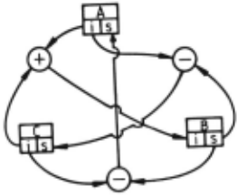
Thus, one can use the value of SUP(B)- INF(C) as an estimated upper bound for A, etc. These relationships are used to create the network for this single inequality, which is shown in Figure 1. As new bounds on B are computed, perhaps from other relationships, they propagate through the network to help compute new bounds on A and c.

There are two advantages to the network structure. First, because values propagate, local improvements in estimates propagate to help constrain other values elsewhere. Even for just local problems, con­ tinued propagation until convergence produces better results than the symbolic methods of ACRONYM. Second, these networks have a nat­ ural wide-scale parallel structure (e.g. 1000+) that might eventually lead to extremely fast evaluation. One disadvantage is that all bound­ ing relationships must be pre-computed as the network is compiled, whereas the symbolic approach can be opportunistic when a fortuitous set of constraints is encountered.

For a given problem, the networks can be complicated, particularly since there may be both exact and heuristic bounding relationships. For example, the network expressing the composition of two 3D refer­ ence frame transformations to give a third contains about 2000 function nodes (of types'+','-', '*', '/', 'sqrt', 'max', ':2:', 'if', etc.). Though the network is formulated for parallel evaluation, simulated serial evalua­ tion is also fast, because small changes are truncated to prevent trivial propagations, unlike in other constraint propagation approaches (see Davis 1987). Convergence is guaranteed (or inconsistency detected) because bounds can only tighten (or cross) and there must be a mini­ mum change for propagation to occur.

3 Geometric Reasoning Networks

The key geometric reasoning data type for high-level computer vision is the position, that represents the relative spatial relationship between two visual features (e.g. world-to-camera, camera--to-model, or model­ to-subcomponent). A position consists of a 3-vector repres~nting re.la.­ tive translation and a unit quaternion (4-vector) representmg relative orientation (of the form (cos(ll /2) , sin(ll/2)w) for a rotation of II about the axis w).

The key geometric relationships concern relative position and have two forms - exact and partially constrained. An example of an exact form is: let object A be at global position Ta-A = (rA, t:.,), (rotation rA and translation fA) and object B be at TA-B= (rAB,t:.,B) relative to A. Then, the global position of B is:

where * is the quaternion multiplication operator and · 1 · is the quater­ nion inverse operator.

A partially constrained position is given by an inequality constraint:

which means that the z component of A's global position is at least 50. Such a constraint might arise from some a priori scene knowledge, or from observation of a fragment of a surface.

Other relationships concern vectors or points linked by a common transformation, as in Tih = ~. or the proximity of points or vectors:

Sets of these constraints are generated as recognition proceeds.

Next, we would like to estimate the values of the constrained quan­ tities (e.g. object position) from the known model and data values and their relationships from a set of constraints. Alternatively, we would like to determine that the set of constraints is inconsistent, so that the hypothesis can be rejected.

A complication is that each data measurement may have some error or uncertainity, and hence the estimated values may also have these. Or, a variable may be only partially constrained in the model or by a priori scene information. Hence, each numerical quantity is represented by an interval and is bounded using the network methodology described in section 2.

The creation of the networks is time-consuming, requiring a sym­ bolic analysis of the algebraic inequalities. Fortunately, there is a nat­ ural modular structure arising from the types of problems encountered during scene analysis, where most geometric constraints are of the type described above. Hence, it is possible to pre-compile network modules for each relationship, and merely connect a new instance of the module into the network as scene analysis proceeds. To date, we have identified and implemented network modules for:

SS - two scalers are close in value

PP - two points are close in location

VV - two vectors point in nearly the same direction

DOT3 - the dot product of two 3-vectors is above a scaler

UNITS - enforcing a unit 3-vector constraint

UNIT4 - enforcing a unit 4-vector constraint

TP - a transformation links a pair of points

TV - a transformation links a pair of vectors

TV2 - a transformation links two pairs of vectors

TT - a transformation maps from one position to a second by a third relative position

P2V - a vector can be defined by two points

QWII - a quaternion is equivalent to an axis and an angle

For example, the UNITS module is defined by the following con­ straints between the components of a vector (p., , p 11 , Pa):

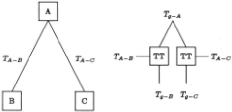
We now include a simple example of network use. Suppose sub­ components B and C are rigidly connected to form object A. Given the estimated positions of the subcomponents in the global coordinate sys­ tem, Ta-B and Ta-Co and the transformations between the object and subcomponent coordinate systems, TA-B and TA-Co then these can be used to estimate the global object position, Ta-A, using two instances of the "TT" module listed above. Figure 2 shows this network. Notice that each subcomponent gives an independent estimate of Ta- Ao so that the network keeps the tightest bounds on each component of the position. Any tighter resulting bounds then propagate back through the modules to refine the subcomponent position estimates.

Rigid Subcomponent Hierarchy Corresponding Geometric Network

4 Binding Degrees of Freedom

Binding degrees-of-freedom is a typical visual geometric reasoning prob­ lem, such as finding the positional parameters, as above. Another ex­ ample is estimating an intrinsic linear degree-of-freedom; as in a pris­ matic robot joint. Its underconstrained position can be modeled by using a variable in the reference frame translation. Then, bounds on this variable can be estimated by using the network method to compute its reference frame relationship relative to its main object.

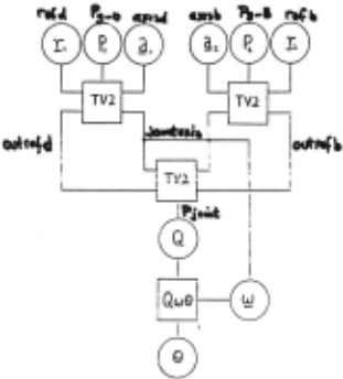
The more difficult case is a rotational degree-of-freedom, as in a robot revolute joint, which we now consider in more detail. The prob­ lem with this case is that there is no element of the rotation specification that exactly corresponds to the degree-of-freedom (unlike the transla-­ tion case) . Fortunately, the cos(ll /2) component of a quaternion can be related to a joint's rotation. Figure 3 shows how to exploit this cos(ll /2) relationship in a subnetwork that solves the problem.

The key subcomponents are B and D, with their estimated global positions Ta-B and Ta-D . From the model, we know which vector in each of their local reference frames is the axis of rotation ( axisb and axisd). Also, from the model we have reference vectors, re/b and refd, such that when they are aligned, the rotation is aero. These two positions and four vectors are inputs into the joint angle subnetwork, at the top of figure 3.

The two TV2 modules at the top map each pair of model vectors to a corresponding pair of scene vectors. Two of these map to the common axis vector. From these we can estimate the joint rotation in quaternion rotation form. This is done by the third TV2 module in the middle of the network. It rotates the global outrefb vector to the global outrefd vector, while maintaining the direction of the global axis vector jointazia.

Finally, to extract the joint angle itself, we use a QW9 module that maps a rotation quaternion to a (9, w) axis-angle form. Here, vector w is also the same as the global rotation axis j ointazia, so this helps the module. {The angular output is given in the form co8(9)).

The following is an example of the joint network:

with very small intervals {0.00001 width) correctly gives an estimated rotation: cos{9) = [0.863, 0.864].

0

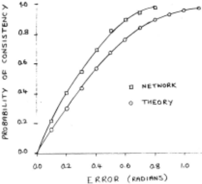
Figure 4: The probability of consistency as a function of E

5 Detecting Inconsistency

The bound estimation algorithm is an incomplete decision procedure. If a network is inconsistent (IN F(V) > SU P(V) for any variable V) then there is definitely no solution. However, a consistent network does not guarantee that a solution exists. This is a problem because the network's ability to detect inconsistent sets of constraints relates to the vision program's ability to reject incorrect hypotheses. We would therefore like to investigate two questions about sets of constraints that have no solution but that nevertheless lead to consistent networks: { 1) how likely are such problems and {2) typically "how close to being soluble» are they.

As our test case we take the problem of finding the rotation that maps a pair of 3D model direction vectors into a corresponding pair of 3D image vectors. This is not only a typical problem in geometric rea.. soning but also a basic one in that other constraints involving multiple matched pairs of directions and locations can be solved by decomposing them into one or more problems of this sort. For our present purposes we assume that the model vectors are known precisely while the image vectors are known only within certain errors. We further assume the errors are isotropic, that is, a nominal vector iJ is enclosed within an error cone of internal angle E to yield the interval vector < iJ, E >I.

A solution exists only if the model vectors can be rotated to lie within the error cones of their corresponding image vectors. Let ih and ~ be the (exact) model vectors and < iJ\., E >I and < %, E >I be the (inexact) image vectors with isotropic error E radians. Then a solution exists if:

For different values of E we estimate the probabilities that randomly chosen vectors, will result in a soluble problem and consistent network by performing many trials. The results are shown in the graph of figure 4. The squares show the probability of network convergence while the dots show the probability of generating a soluble problem. The latter can be calculated analytically and is shown by the curve in figure 4 which is the function:

The probability of the network being inconsistent given that the prob­ lem has a solution is zero for any value of E, but the probability of the network being consistent when no solution exists is significant as figure 4 shows.

We now define:

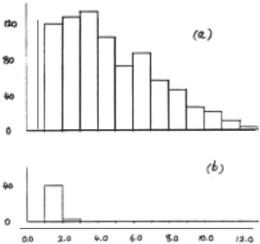
as a measure of "distance from solution». The problem is soluble iff 8 ~ 1. For values of s larger than but close to 1 the problem is ·only just» insoluble. By again performing many trials {for fixed E = 0.1) we compiled histograms of values for 8 in trials that were predicted by the above to have no solution and led to a network state that was (a) inconsistent or (b) consistent. The results are shown in figure 5.

Figure 5 part (a) shows that there is a wide distribution of 8 values between 8 = 1 and 8 = 12 for insoluble problems correctly detected by the network. On the other hand, part (b) shows that insoluble problems that the network could not detect are concentrated mostly between 8 = 1 and 8 = 2 and are consequently close to being solu­ ble. We therefore conclude that the network will not give misleading results when problems are far from solution and that in practice the incompleteness problem has only a limited effect.

6 Propagation of Uncertainty

Because each numerical quantity is represented as an interval, and be­ cause most geometric calculations involve several arithmetic functions, it is possible for error intervals to grow as they propagate through the network. Hence, we examine some of the numerical performance of the network modules. This section discusses results for two key modules, TT and TP, and the joint angle estimation network.

By examining the algebraic relationships involved in the composi­ tion of reference frame module (TT), it can be shown analytically that if each orientation component of a random position Ta-b has error 6 and each orientation component of a random position Tb-c has error E, then each component of the resulting position Ta-c = Ta-b · Tb-c has (statistical) error:

assuming that both 6 and E are small. This result has been verified by simulation. Figure 6 shows the empirical results, which taper off as the maximum error volume is reached. In essence, the results mean that the output error width is about 1.7 times the input error width.

A similar analysis of the transformation of a location (TP module) shows that each translation component has output error:

where E is the input rotation quaternion error on each component, and L is the distance of the input point from the origin. This is sensible, because small rotation errors amplify along a long baseline, to produce larger translation errors. This result has also been verified empirically.

We have not found an analytic form for the error in joint angle estimation, as a function of input position error, but empirical results show that the output error varies approximately linearly with input error and has magnitude about 5.5 times as big. The results were generated by perturbing each component of T 11 _s and Tg-D by an error E for a randomly chosen rotation, and then looking at the output error of the co.!(ll) rotation estimate. The results also show that the error reaches a maximum when the input error reaches about E = 0.18, so the input positions need to be somewhat constrained for joint angle estimation to work.

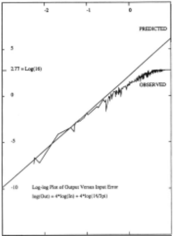
. Figure 6 also show that there is some variability in the results (be­ stdes the underlying trend) which is undesirable. One contributor to the problem is several special cases to the TV2 module that solve for the rotation using a different set of bounds from the main case and hence have different numerical properties. '

7 A Large Network Example

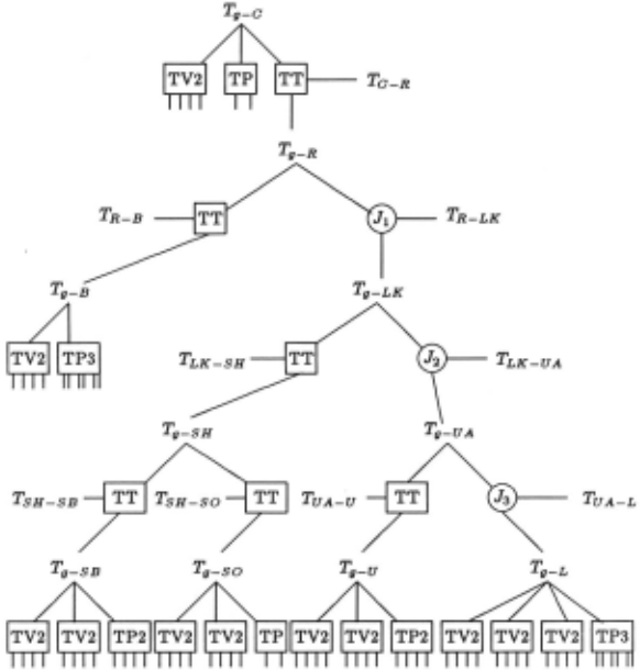
Figure 8 shows the full network generated for analy~ing the position of a robot in a test scene. As before, the boxes represent transfor­ mations, but there are more types used here. The TPn boxes stand for n instances of a TP module. The circular "Jn· boxes represent three identical instances of subnetworks allocated for transformations involving joint angles, which are omitted to simplify the diagram (each contains 7 network modules). The core of the subnetworks was shown in figure 3, but some additional modules are added to align reference frames. The relative positions of objects are given by the T structures, such as T 11 -R, which represents the position of the robot in the global reference frame . These are linked by the various transformations. Links to model or data vectors or points are represented by the unconnected segments exiting from some boxes.

The top position T 11 - c is the position of the camera in the global coordinate system, and the subnetwork to the left and below relates features in the camera frame to corresponding ones in the global co­ ordinate system. Below and right is the position Tg-R of the robot in the global coordinate system and the position Ta-R, of the robot in the camera coordinate system, all linked by a TT position trans­ formation module. Next, to the bottom left is the subnetwork for the cylindrical robot body Tg-B· The "J1" node connects the robot posi­ tion to the rest ("link") on the right, whose position is Tg-LK· Its left subcomponent is the rigid shoulder ASSEMBLY (SH) with its subcom­ ponents, the shoulder body (SB) and the small shoulder patch (SO). To the right, the "J2" node connects to the "armasm· ASSEMBLY (UA), linking the upper arm (U) to the lower arm (L), again via another joint angle (J3). At the bottom are the modules that link model vectors and points to observed surface normals, cylindrical axis vectors, and central points, etc. Altogether, there are 61 network modules containing about 96,000 function nodes.

The network structure closely resembles the model subcomponent hierarchy, and only the bottom level is data--dependent. There, new nodes are added whenever new model-to-data pairings are made, pro­ ducing new constraints on feature positions.

Evaluating the complete network from the raw data requires about 1,000,000 node evaluations in 800 "clock-periods" (thus implying over 1000-way parallelism) . Given the simplicity of operations in a node evaluation, a future machine should be able to support easily a 1 mi­ crosecond cycle time. This suggests that an approximate answer to this complicated problem could be achieved in about one millisecond.

Because the resulting intervals are not tight, confidence that the mean interval value is the best estimate is reduced, though the bounds are correct, and the mean interval values provide useful position es­ timates. To tighten estimates, a post-processing phase progressively shrinks the bounds on the intervals. Each position variable was ex­ amined to see if its interval was tight . H not, it was reduced in size by 10% and the new bounds were then allowed to propagate through the network. For the robot example, this required an additional 12,000 cycles, implying a total solution time of about 13 milliseconds on our hypothetical parallel machine.

Using the geometric reasoning network, the numerical results for the whole robot in the test scene are summarized in Table 1. Here, the values are given in the global reference frame rather than in the camera reference frame.

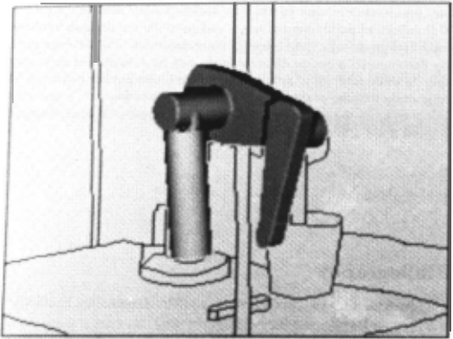
The results of the position estimation can been seen more clearly if we look at Figure 7, that shows the estimated robot position overlaying the original scene. Now, we are using the camera position of the whole robot assembly plus the estimated joint angles from above. While the positions of the individual components are reasonable, the accumulated errors in the position and joint angle estimates cause the predicted position of the gripper to drift somewhat from the true position. The iterative bounds tightening procedure described above produced this result, which was slightly better than the one-pass method.

8 Discussion

We have seen how the network methods can detect inconsistency and es­ timate degrees-of-freedom. From the examples given, it is obvious that this network approach can solve complex geometric reasoning problems, has an incremental modular structure and has potential for wide-scale parallelism. Unfortunately, after experience with use of the network approach, it has become obvious that there are also problems, partic­ ularly when working with noisy data.

One inherent problem concerns the ambiguity in the quaternion ro­ tation representation, as the rotation (q0 , q1 , ~. q3 ) is equivalent to the rotation (-qo, -q1 , -~, -q3 ) . When coupled with the interval arith­ metic, sometimes the bounds on terms cannot choose between alterna­ tives, producing unnece88arily large bounds. For example, the qo term may acquire a bound [-a-£, +a+ t], when the bound [+a-£, +a+ t] may be equally satisfactory. It is not po88ible to require that q0 ~ 0 always, because the composition of some rotations satisfying this con­ dition may produce a rotation that violates this (using the standard quaternion rotation formulation) . A related problem also occurs with a tolerance £ about qo terms near one, creating intervals [1- £, 1] and [-1, -1 + £].

These problems suggest that the model-based reasoning program may have to analyse the results and occasionally split or introduce al­ ternative cases, given an understanding of the representation problems ..

While the error analysis given in section 6 showed that errors usually do not grow too quickly, when we look at the robot network (Figure 8), we still find a problem. In particular, it turns out that the chain of reference frame transformations from the robot in the global reference frame (T.,_R) to the data vectors involved in the lower arm position (below T.,-L) involve ten TV2 and three TT modules. A88uming each has an output interval width of 1. 7 times the input interval width means that the combined contribution of the lowerarm evidence to the robot has an error interval width of (1.7)1 3 = about 1000 times the input error interval. As the maximum output interval can be only [-1,+1] for the rotation, this implies that the input uncertainity can be at most about 0.01, which is unreasonably strict.

However, this error analysis must also consider that many of the reference frame transformations are the identity transformation, which create little error (and need not even be introduced into the network) . Further, though the estimates may not propagate all the way to the robot global position node, they will help constrain more closely linked structures.

It should be noted that geometric reasoning involving a multiple joint articulated object is a genuinely complicated problem, whereas most object recognition problems have a much flatter model hierarchy, involving fewer compound degrees-of-freedom, if any at all.

A final problem posed by the interval approach is that of finding the "best· estimate for a parameter, when the intervals are large, partic­ ularly with rotation parameters. While integrating enough randomly distributed errors will cause the widths of the intervals to converge to a "correct· answer, we seldom have more than a few measured values (e.g. surface normals, curvature axes) . Consequently, a statistical tech­ nique (e.g. Durrant-Whyte 1987) or a final least-squared error position refinement step also seems attractive, though they might have problems handling rotational degrees-of-freedom.

Though research on the efficient use of these networks is continu­ ing, problems overcome by the new technique included the bounding of transformed parameter estimates and partially constrained variables and effective detection of geometric inconsistencies. The network mod­ ule decomposition means that networks can be constructed incremen­ tally as scene analysis proceeds. The network also has the potential for large scale parallel evaluation. This is important because a consider­ able portion of the proce88ing time in three dimensional scene analysis is spent doing geometric reasoning.