
A "Small Leakage" Model for Diffusion Smoothing of Image Data
Proceedings of the Eleventh International Joint Conference on Artificial Intelligence. Vision and Robotics. Pages 1585-1589.
© 1989 International Joint Conferences on Artificial Intelligence
Abstract
In this paper, an implicit numerical scheme of diffusion smoothing is given for both intensity and depth images, which uses a changeable time step to reduce the computation. Emphasised is a "small leakage" diffusion model as an efficient way to maintain both boundary position and curvature signs along the surface boundary in smoothing, which will be useful for approximation and segmentation of sculptured surfaces.
- [Ames, 1977] Ames, W.F., Numerical Methods for Partial Differential Equations, 2nd ed. Academic Press, New York, 1977, pp.47. Babaud eta/., 1986]
- Babaud, J., Witkin, A.P., Baudin, M. and Duda, R.O., Uniqueness of the Gaussian Kernel for Scale-Space Filtering, IEEE Transactions on Pattern Analysis and Machine Intelligence, Vol. PAMl-8, No. 1, 1986.
- [Besl and Jain, 1986] Besl, P., and Jain, R.C., Invariant Surface Characteristics for 3D Object Recognition in Range Images, Computer Vision, Graphics, and Image processing, 33, 30-80, 1986.
- [Brady et a/., 1985] Brady, M., Ponce, J., Yuille, A. and Asada, H., Describing Surfaces , MIT A.l. Memo 822, 1985.
- [Cai, 1987a] Cai, L.D., Diffusion Smoothing on Dense Range Data, DAI WP-200, Department of A.I., University of Edinburgh, 1987.
- [Cai, 1987b] Cai, L.D., Some Notes On Repeated Averaging Smoothing, DAI RP-337, Department of A.I., University of Edinburgh, 1987. Also in Proc. of BPRA 4th Int. Conf. on Pattern Recognition, Cambridge, U.K., 1988, Lecture Notes in Computer Science, J.KiUler (Ed.), Vol. 301, Springer-Verlag. pp. 596-605.
- [Canny, 1983] Canny, J.F., Finding Edges and Lines in Images, MIT A.I. Tech. Repon 720, 1983. pp. 72-75.
- [Feng et a/., 1978] Feng, K. et al. (Ed.), Numerical Computation methods (in Chinese), Defence Industry Press, 1978. pp. 489-509.
- [Gourlay, 1985] Gourlay, A. R., Implicit convolution, Image and Vision CompUiing, Vol. 3 No. 1, 1985.
- [Koenderink, 1984] Koenderink, J.J., The Structure of Images, Biological Cybernetics 50, 1984. pp. 363-370.
- [Ponce and Brady, 1987] Ponce, J. and Brady, M., Toward a Surface Primal Sketch, in Three-Dimensional Machine Vision, T.Kanade (Ed.), Kluwer Academic Publishers, 1987. pp. 225-227.
- [Rosenfeld and Kak, 1976] Rosenfeld, A. and Kak, A.C., Digital Picture Processing, 1nd ed., Academic Press, New York, 1976. pp. 184.
- [Terzopoulos, 1985] Terzopoulos, D., Computing Visible-Surface Representations, MIT A.I. Memo No. 800, 1985, pp. 12-17.
- [Witkin, 1983] Witkin, A., Scale-Space Filtering, in Proc. of 7th Int. Joint. Conf of Artificial Intelligence, Karlsruhe, 1983. pp. 1019-1021.
- [Yuille and Poggio, 1983] Yuille, A.L. and Poggio, T., Scaling Theorems for Zero Crossings, MIT A.l. AIM-722, 1983.
References were extracted automatically from the PDF and may contain errors.
Full text extracted automatically from the PDF; figures, tables and equations may differ. The PDF is the version of record.
1 Introduction
In early visual processing, Gaussian convolution (smoothing) is well suited for reducing image noise owing to its elegant properties [Yuille and Poggio, 1983]. A widely used and efficient algorithm of Gaussian convolution in computation is the repeated averaging smoothing [Brady el al., 198S],[Canny, 1983]. As an equivalence to Gaussian convolution, diffusion smoothing has also been investigated by many papers [Rosenfeld and Kale, 1976],[Koenderink, 1984],[Gourlay, I98S],[Babaud el al., I986],[Cai, I987a,b],.
There are two problems for the effective application of diffusion smoothing: the first is to construct an efficient algorithm; and the second is to treat the boundary condition properly according to different requirements. For the first problem, [Cai, I987a] proposed an implicit algorithm (DISCI) to complete diffusion smoothing with a lower computational complexity than Gaussian smoothing's; and [Cai, I987b] further showed that the repeated averaging smoothing mask (as well as some other masks) can be easily derived from the explicit diffusion smoothing. For the second problem, a "small leakage" diffusion model is proposed in this paper as an efficient way to maintain both boundary position and curvature signs along the surface boundary in smoothing.
2 Gaussian Convolution and Diffusion Equation
Given a diffusion (or heat conduction) equation:
where u (x ,y ,I) is the temperature distribution on domain D (x ,y) at time 1 , f (x ,y) is its initial value; b is the heat conduction coefficient and .0. = aa 2 2 + ~ is the Laplacian operator. X ey
As is well known, the solution of equation (I) is just the Gaussian convolution off (x ,y ):
with a substitution
where * denotes the convolution operator, expO is the exponential function, and cr is the smoothing scale parameter.
3 DES: An Explicit Numerical Scheme of the Diffusion Equation
Discretising diffusion equation (1.1) at eight neighbouring nodes around the central node (i J) and time k, we can get the following explicit numerical scheme:
where i = 0 (I) M denotes that i runs from 0 to M in unit step; ui 1 J denotes the difference equations' solution u at the node (ih Jh) and time 1 = k't, which corresponds to the diffusion equation's solution u (x ,y ,I) at the same node and time; h is the spatial step, 't is the time b't step and~= 2 . h
Setting 't=I and h=1 in (4) yields a varies of 3x3 square masks corresponding to different values of diffusion coefficient b , by which the square mask of repeated averaging smoothing in [Brady el al., 1985] is shown as a special case of the diffusion smoothing [Cai, 1987b].
Applying Fourier separation method [Feng et al., 1978],[Ames, 1977] to this explicit scheme (4) gives the following stability condition:
Using any 't beyond this stability range leads to the computational errors be amplified in the smoothing and yields pointless results.
4 DISCT: An Implicit Numerical Scheme of the Diffusion Equation
To efficiently solve the diffusion equation (!), an implicit numerical scheme in [Feng, 1978] is adopted as below:
where
Note that A is a tridiagonal and diagonal-dominant matrix, thus the linear algebra system (7) can be easily solved with a numerically stable computation.
Furthermore, not like the explicit diffusion smoothing, the implicit diffusion smoothing scheme is unconditionally stable in computation, hence there is no constraint to the time step. Owing to this novel property, a larger even changeable time step is allowed, which makes the Diffusion Implicit Smoothing with Changeable Time step scheme (DISCT) efficiently reduce the computation.
For example, when smoothing an image with a single scale 0', the computational complexity of Gaussian convolution is 0(160'M~. From (3), the diffusion time interval should be [0, ~ ], and the complexity of DISCT scheme is only 0(10(20'-1)M 2 ) when using a changeable time 2k+1 k 2 (k+1f step 't="""4b in each sub-interval [ 2b ·--u;-], k~l.
When smoothing in multi-scale space [Witkin, 1983], the complexity of Gaussian convolution is raised to 0(8cr(cr+1)M~. but the complexity of DISCT remains the same 0(10(20'-1)M 2 ) [Cai, 1987a], where 0' is the maximal scale.
5 Diffusion Smoothing Without Boundary Preservation
When DISCT is to be applied without boundary preservation, as is common for smoothing an intensity image, the computation can be further reduced by first merging all left hand and right hand column vectors in (7.x) into two MxM matrices then solve the matrix equation as whole; similarly treat the row vectors in (7.y):
The computational complexity is therefore reduced to O(crM)!
(9) 6 Treatment of the Surface Boundary
Depth image smoothing is somewhat different from many cases of intensity image smoothing. In a depth image, an object usually has an obvious boundary which will be blurred by smoothing if without boundary preservation.
where, and hereafter [ · · · f denotes the transpose operation of a row vector or a matrix.
The initial position of the surface boundary can be fixed as a "boundary condition", however, it is of liule avail since the reduction of depth contrast along the surface boundary leads to the surface gradually "melting" into the background in smoothing [Ponce and Brady, 1987], particularly, in multi-scale smoothing. A feasible boundary treatment is thus required to preserve the surface boundary.
which can be represented in a matrix form:
There are several ways to prevent the surface boundary "melting" into the background. For instance, the "computational molecules" technique [Terzopoulos, 1985) is adopted in the repeated averaging smoothing [Brady et al., 1985]; and, similarly, "one pixel horizontal extension" of the surface boundary is used in diffusion smoothing [Cai, 1987a).
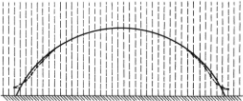
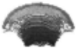
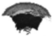
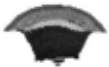
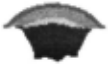
However, under the above treatments, the depth variation at the boundary is not consistent with that in the inner area. As shown in Figure 1, the depth at a cylindrical surface boundary will not be reduced but be raised while the depth in the inner area is decreased, which makes the marginal area of surface flatten rapidly and change the surface concavity/convexity there. This tendency will further propagate to the central area during the smoothing process until the whole surface becomes flat. So Gaussian CO!Jvolution in 2.5-D space cannot preserve the shape of a cylindrical surface as it does in 3-D space [Brady et al., 1985), nor the diffusion smoothing with "one pixel horizontal extension" boundary treatment Both of them will introduce a side-effect: the signs of curvatures (Gaussian curvature and mean curvature) at many pixels along the surface boundary might be changed although the surface boundary position now can be maintained in the smoothing process.
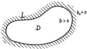
From the viewpoint of diffusion smoothing, this effect can be explained intuitively with a "no leakage" diffusion (heat conduction) model shown in Figure 2., where "no heat energy on the domain D will leak out through the boundary L which is surrounded by some absolutely heat-isolated medium whose heat conduct coefficient b0 is zero." Hence, when the temperature distribution finally becomes flat, it will not be a zero-flat one on the whole x-y plane as in the case of surface smoothing without boundary preservation but will be a non-zero flat one over the domain D . The value of the final flat distribution will be higher than the initial (depth) value at the boundary and lower than that in the central area, which leads to the above surface distortion.
To avoid introducing errors of curvature signs near the boundary, [Ponce and Brady, 1987) suggested smoothing in intrinsic coordinates that "instead of smoothing z, the surface point is moved along its normal a distance that depends upon the projected distances of the point's neighbours from the tangent plane." This method is expensive in computation as it needs calculating all normal vectors on the surface.
To maintain both the boundary position and curvature signs along the surface boundary, we propose a modified diffusion model - the "small leakage" model to treat the boundary pixels: a small part of heat energy is allowed to be leaked out to an ideal good conductor through a thin, partially heat-isolated medium at the slant boundary so that the depth of, e.g., a cylindrical surface boundary will be slightly reduced rather than being raised, whereas no heat energy is leaked out through the horizontal surface boundary. Therefore, both the boundary position and surface shape can be preserved at most of pixels along the surface boundary.
Speaking mathematically, the "small leakage" model applies a so called "natural boundary condition"
to the diffusion equation ou lot = b Ll.u shown below:
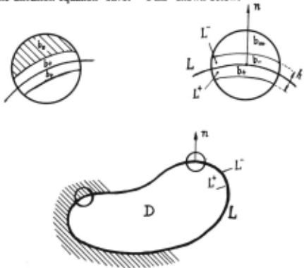
Where D is the surface domain; L is the boundary of D , L + is the internal side and L -, the external side; n is the outward normal vector at the boundary L; b is the heat conduction coefficient: b + for the surface material, e.g. 0.5, b_ for the thin heat-isolated medium, about 10% of the b+, e.g., 0.05, and b_ for ideal heat conductor.
This means the heat conduction coefficient b has a discontinuity across the surface boundary and different media; so does the temperature gradient ~~ . Meanwhile, the heat energy exchanged across the boundary is always continuous due to the law of conservation of energy.
In practice, to avoid computing the normal vector at each boundary pixel, this natural boundary condition is further simplified. It is split into x- and y-directions respectively as follows:
we obtain their vector forms as below:
Obviously, these coefficient vectors are compatible with the DISCT scheme's tridiagonal coefficient matrix (8). Hence, when the natural boundary condition is applied to a diffusion equation, only a small revision to A corresponding to the slant boundary pixels is needed, and it requires little computation. Matrix A is still a diagonal-dominant one and the lower computational complexity of the DISCT algorithm in [Cai, 1987a] is still available.
7 Experimental Results and Further Work
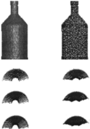
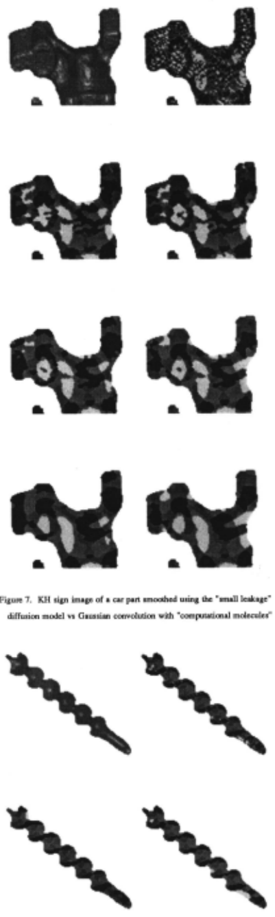
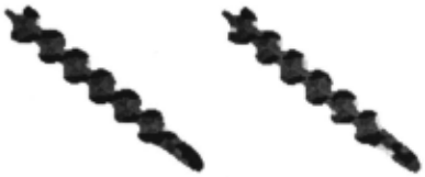
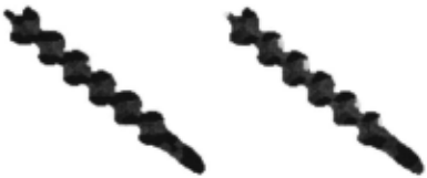
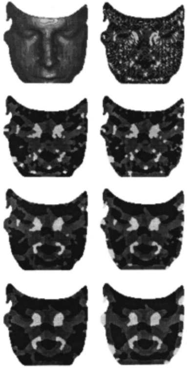
Six figures are shown in this section as the experimental results of the range data processed in scale space using the "small leakage" diffusion smoothing and the Gaussian smoothing with "computational molecules", where the diffusion time t = 0, 1, 4 and 9 correspond to Gaussian scale cr = 0, 1, 2 and 3.
Figure 4 is for a cylindrical oil bottle and Figure 5 is for a light bulb, where the side-view is used to compare the smoothing effects at the boundary. Figure 6 is for the same light bulb, but using KH sign image [Besl and Jain, 1986] to compare the results from both smoothing methods. Similar are the rest three figures for a Renault car part, a drill and a human face using respectively. Each grey level in the KH sign image corresponds one of the eight surface types listed in Table 1.
In each figure, the object from raw data is shown at the top part, where the left side is for cosine-shading image and the right side for KH sign image; the smoothed objects are shown at the rest parts, where the left sides are for KH sign images from "small leakage" diffusion
At the boundary pixel (ij), discretising the x- and y-directional gradients at time k+t and k+1 respectively:
smoothing and the right sides for KH sign imges from Gaussian smoothing.
As is shown in these figures, Gaussian smoothing with the "computational molecules" technique introduces undesired changes in curvature sign in the marginal area, which forms. a strip along the surface boundary which expands along with the increment of the scale; whereas diffusion smoothing with the "small leakage" model preserves the curvature signs quite well along the surface boundary, which will be very helpful for approximation and segmentation of sculptured surface.
A better result might be expected by using a diffusion model with a piecewise continuous coefficient b{x,y) over the whole xy-plane. Experiments on how to construct such a function b(x,y) are still in progress.

Acknowledgements
This research is funded by the University of Edinburgh. Thanks are given to Dr. R.B. Fisher for supervision and R.M. Cameron-Jones for discussion.
@inproceedings{ijcai1989p252,
  title     = {A "Small Leakage" Model for Diffusion Smoothing of Image Data},
  author    = {Cai, Li-Dong},
  booktitle = {Proceedings of the Eleventh International Joint Conference on
               Artificial Intelligence, {IJCAI-89}},
  publisher = {International Joint Conferences on Artificial Intelligence},
  editor    = {N. S. Sridharan},
  pages     = {1585--1589},
  year      = {1989},
  month     = {8},
  note      = {Vision and Robotics},
  url       = {https://ijcai.org/proceedings/1989/252},
}
TY - CPAPER TI - A "Small Leakage" Model for Diffusion Smoothing of Image Data AU - Cai, Li-Dong T2 - Proceedings of the Eleventh International Joint Conference on Artificial Intelligence, IJCAI-89 PB - International Joint Conferences on Artificial Intelligence PY - 1989 SP - 1585 EP - 1589 UR - https://ijcai.org/proceedings/1989/252 ER -Copied
Machine-readable versions of this paper, for tools and AI agents:





