Perception of Non-Rigid Motion: Inference of Shape, Material and Force

1 Introduction

Non-rigid motion seems to be ver_y comple~. _When ~n object is struck so that it moves m a non-.rigid, . elastic manner each point on the surface goes off m a different directio~ . It seems, therefore, that a full description of non-rigid motion must have even more degrees of free­ dom than a full description of shape. Despite this ap­ parent complexity, however, people ar~ often abl~ to~­ curately predict the time course of obJects expenencmg non-rigid behavior, and are even able to infer material properties from observing such motion. . .

For instance, people can watch a tree hmb swaymg in the wind and make a good estimate of its stiffness, strength and mass. More commonly, when someone wants to deteri:nine the properties of an object they poke at it to see and feel it deform, and tap it to hear it res­ onate. From these visual, tactile, and auditory cues we are somehow able to ascertain material properties.

In this paper we will examine the finite element method of simulating the dynamics of collisions, and show that it can be decomposed into simple, closed-form differential equations describing the object's vibration modes. We will then show that for most objects under most conditions a relatively small number of modes are required to accurately describe how the object deforms as a function of time. Finally, we will show that for simple collisions we can estimate the object's m~teri~l properties by observing these vibration modes usmg Vi­ sual, tactile or even auditory data.

·This research was made possible by National Science Foundation Grant No. IRI-87-19920 and by ARO Grant No. DAALOJ-87-K-0005

2 Background: The Finite Element Method

The finite element method (FEM) is a technique for sim­ ulating the dynamic behavior of an object. In the FEM the continuous variation of displacements throughout an object is replaced by a finite number of displacements at so-called nodal points. Displacements between nodal points are interpolated using a smooth functio~ . E?­ ergy equations (or functionals) can then be derived m terms of the nodal unknowns and the resulting set of simultaneous equations can be iterated to solve for dis­ placements as a function of impinging fo~ces. In the dynamical case these equations may be wntten:

where u is a 3n x 1 vector of the ( x, y, z) displacements of the n nodal points relative to the objects' center of mass M D and K are 3n by 3n matrices describing the dtass: damping, and material stiffness between e~ch point within the body, and f is a 3n x 1 vect~r descnb­ ing the ( x, y, z) components of the forces actm~ o~ the nodes. This equation can be interpreted as assignmg a certain mass to each nodal point and a certain mate­ rial stiffness between nodal points, with damping being accounted for by dashpots attached between the nodal points. The damping matrix D is normally taken to be equal to s1M + s2K for some scalars s1, s2 . When s1 :j= 0, s2 :j= 0 this is called Raleigh dampi~g, for s2 = 0 it is called mass damping, and for s1 = 0 stiffness damp­ ing.

To calculate the result of applying some force f to the object one discretizes the equations in tiJ?e, pick~ng an appropriately small time step, solves this equ_a_twn for the new u and iterates until the system stabihzes. ' 0 0 Direct (implicit) solution of the dynamic equatwns. requires inversion the K matrix, and i~ t_hus computation­ ally expensive. Consequently exphcit Eu!er. met~ods (which are less stable, but require no matnx mverswn) are quite often applied. . .

Even the explicit Euler methods are qmte expensiVe, because the matrices M, D, and K are quite large: for instance, the simplest 3-D parabolic element produces 60 x 60 matrices, corresponding to the 60 unknowns in the 20 nodal points (xi, Yi, zi) which specify the element shape. In most situations M, D, and K are very much larger than 60 x 60, so that typically hundreds or thou­ sands of very large matrix multiplications are required for each second of simulated time. For more details see references [1 ,2].

3 Modal Analysis

Because M, D and K are normally positive definite symmetric, and M and D are assumed to be related by a scalar transformation, :Equation 1 can be transformed into 3n independent differential equations by use of the whitening transform, which simultaneously diagonalizes M, D, and K . The whitening transform is the solution to the following eigenvalue problem:

where A and ljJ are the eigenvalues and eigenvectors of M- 1 K.

Using the transformation u = l/Ju we can re-write Equation 1 as follows:

In this equation q,T M l/J, q,T Dp, and q,T K ljJ ~re dia~onal matrices, so that if we let M = q,T M l/J, D = ljJ DljJ, f< = q,T K l/J, and f = q,T f then we can write Equation 3 as 3n independent equations:

where Mi is the ith diagonal element of M, and so forth . Because the modal representation diagonalizes these matrices it may be viewed as preconditioning the mass and stiffness matrices, with the attendant advan­ tages of better convergence and numerical accuracy.

What Equation 4 describes is the time course of one of the object's vibration modes, hence the name modal analysis [3]. The constant Mi is the generalized mass of mode i, that is, it describes the inertia of this vibra­ tion mode. Similarly, [Ji, and f<i describe the damE_ing and spring stiffness associated with mode i, and /i is the amount of force coupled with this vibration mode. The ith row of ljJ describes the deformation _the object experiences as a consequence of the force /i, and the eigenvalue Ai is proportional to the natural resonance frequency of that vibration mode.

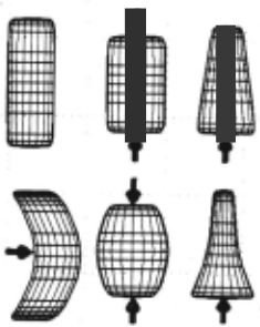
Figure 1 illustrates the some ofthe first and second or­ der modes of a cylinder. Figure 1(a) shows the cylinder at rest , (b) shows the cylinder experiencing a linear de­ formation in response to a compressive force, (c) shows the cylinder experiencing a linear shear deformation in response to an accelerating force , (d) shows a quadratic deformation in response to a centrally-applied (bend­ ing) force, and (e) and (f) show how both the linear and second order deformations can be superimposed to produce a more accurate simulation of the object's re­ sponse to the compressive and accelerating forces shown in (b) and (c) .

To obtain an accurate simulation of the dynamics of an object one simply uses linear superposition of these modes to determine how the object responds to a given force. Because Equation 4 can be solved in closed form, we have the result that for objects composed of linearly­ deforming materials the non-rigid behavior of the object in response to an impulse force can be solved in closed form for any timet . The solution is discussed in Section 4. In environments with more complex forces, however, analytic solution becomes cumbersome and so numerical solution is preferred. Either explicit or implicit solution techniques may be used to calculate how each mode varies with time.

Non-linear materials may be modeled by summing the modes at the end of each time step to form the material stress state which can then be used to drive nonlinear plastic or viscous material behavior.

4 Number Of Modes Required

The modal representation decouples the degrees of free­ dom within the non-rigid dynamical system of Equation 1, but it does not reduced the total number of degrees of freedom. However once decoupled, we can separately analyze the various modes in order to determine which ones are required in order to obtain an accurate descrip­ tion of an object's non-rigid dynamic behavior.

The most important observation is that modes asso­ ciated with high resonance frequencies normally have little effect on object shape. This is because:

• The displacement amplitude for each mode is in­ versely proportional to the square of the mode's resonance frequency. Thus higher frequencies typi­ cally have small amplitudes.

• Damping is proportional to the mode's resonance frequency. Thus higher frequency vibrations dissi­ pate quickly.
• Frequencies are excited in proportion to the fre­ quency content of the input force. The force gen­ erated by simple collisions typically have a roughly Gaussian time course, so that an individual reso­ nance frequency f receives energy proportional to e-1~/u. Thus low frequencies typically receive more energy than high frequencies.

The combination of these effects is that high­ frequency modes have very little amplitude, and even less effect, in simple collisions. As a consequence much more efficient (and still accurate) simulation of an ob­ ject's dynamics can be accomplished by discarding the small, high-frequency modes, and considering only the large-amplitude, low-frequency modes [5,6]. Exactly which modes to discard can determined by examining their associated eigenvalue, which determines the reso­ nance frequency.

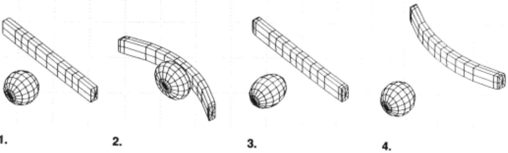
Experimentally, we have found that most common­ place multi-body interactions can be adequately mod­ eled by use of only rigid-body, linear, and quadratic strain modes. Figure 2, for instance, shows a example of a simulated non-rigid dynamic interaction: a ball col­ liding with a two-by-four. As can be seen, the interac­ tion and resulting deformations look realistic despite the use of only linear and quadratic modes. 1 Figure 1 also illustrates how use of linear and quadratic modes can accurately simulate non-rigid motion. Note, however, higher-order modes are required to accurately model the objects whose dimensions differ more than an order of magnitude.

1 Perhaps the most impressive fact about this example, however, is the speed of computation: Using a Symbolics 3600 (with a speed of roughly one MIP), it requires only one CPU second to compute each second of simulated time!

4.0.1 Use of Fixed Modes

Normally, in either the finite element or modal meth­ ods, the mass, damping, and stiffness matrices are not recomputed at each time step. The use of fixed M, D, and K (or, equivalently, fixed modes) is well-justified as long as the material displacements are small . The defi­ nition of "small," however, is quite different for different modes. Because the eigenvalue decomposition in Equa­ tion 2 performs a sort of principal-components analysis, it is the gross object shape (e.g., its low-order moments of inertia) determine the low-frequency modes, which as a consequence are quite stable. High-frequency modes are much less stable because they are determined by the fine features of the object's shape.

In the standard finite element formulation the action of each mode is distributed across the entire set of equa­ tions, so that one must recompute the mass and stiff­ ness matrices as often as required by the very highest­ frequency vibration modes. When these high-frequency modes are discarded the mass, damping, and stiffness matrices need to be recomputed much less frequently. In most situations it is sufficient to use single, fixed set of low-frequency modes throughout an entire simulation.

5 Estimation of Material Properties

Let us imagine that we have seen the image sequence shown in Figure 2, and have been able to compute a full 3-D description of the object's shape at each instant. How can we estimate the material properties of these objects? The first step is to compute for each object a description that decomposes the object motion into its low-order modes.

This can be accomplished by forming the vector p that describes each point on the object's surface, and then computing the matrices M, D, and K matrices using unit values for density and spring constant. Be­ cause these matrices are determined by the vector p up to an overall constant, the eigenvectors found by solving Equation 2 will be identical regardless of the material properties (excepting, of course, non-linearly-behaving materials); only the eigenvalues depend upon the mate­ rial properties. Thus given the object's shape, we can directly determine f/J, the object's deformation modes.

In this straightforward approach the matrices M, D, and K ca.n become quite large, so that solution to Equa­ tion 2 becomes difficult. A more efficient method of de­ termining ifJ is be to fit either an eight or twenty point polygonal model to the sensed data (perhaps by use of the techniques described in reference [2]), and use the values of those points to construct a much smaller vector p. Given eight points we can form M, D, and K ma­ trices that are 24 x 24 in size, and then solve Equation 2 to obtain the object's linear vibration modes. Given twenty points the matrices are 60 x 60, and produce both linear and quadratic vibration modes.

A still more efficient scheme can be obtained by not­ ing that the axes of the object can allow us to directly disentangle the action of the various modes, so that by estimating axis shape and length we can avoid solving Equation 2. This approach is described in more detail below.

Given ifJ and a description p(t) of the object's shape over time, we can directly decompose the object shape into a vector p(to) describing the object's shape at time t = t 0 and the amplitudes u(t) = ¢J- 1 (p(t) - p(t0 )) of each of the individual modes over time. The generic time behavior of each mode ui(t) in response to an im­ pinging force is given by Equation 4. The solution to this equation is

for the overdamped, critically damped, and under­ damped cases, where

and A and B depend on the initial conditions [11] . The third case, underdamped motion, occurs most com­ monly in mechanical systems and is referred to as "damped vibration." To see this we let A = R cos 5 and B = R sin 8 in Equation 5 to obtain

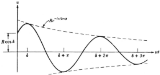
which is graphed in Figure 3(b ).

_

Because the time behavior of iii is a function of Mi , Di and f<i, in simple situations we can recover the phys­ ical parameters of the object's material by measuring iii over time. This is particularly straightforward when the mode is underdamped, as in Figure 3, so that several cy­ cles of deformation occur, because in this case we need only measure the frequency and amplitude of the de­ formation peaks. When the mode is critically damped or overdamped only one peak occurs; however it is still possible to measure the material properties from peaks in the first derivative of the modal amplitude.

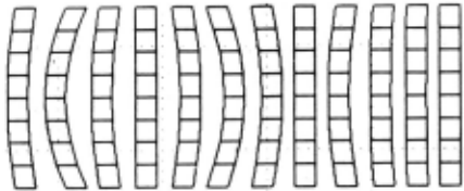
For example, in the sequence of Figure 2 we can ob­ serve the bending of the two-by-four in response to the impact of the ball, as illustrated by Figure 4. If we plot the amplitude of this deformation mode in response to the unknown impact force h (which, without loss of generality, we will take to be of unit time duration), then we will obtain the graph shown in Figure 3. From the succession of peak amplitudes a; = ui(6 + j1r) and the times t; = 6 + j 1r at which these peaks occur we can obtain the following relations:

(8)

These relations are well-conditioned, so that the accu­ racy of the material property estimates will depend pri­ marily on the accuracy with which we can estimate the a; and the t;.

Thus by observing modal amplitude after a sharp im­ pacts we can estimate the force of collision and all of the material's physical parameters, up to a scale factor which is the mass associated with that mode. We note that except for non-linear, visco-plastic materials the relationships in Equations 8 hold exactly for all materi­ als, all vibration modes, and all object geometries; they are approximations only in the sense that finite element analysis is an approximation.

5.1 Estimation of Mass

By tracking geometry over time we can estimate the material properties up to an overall scale constant that depends upon the amount of mass involved in the par­ t icular vibration mode. The obvious question, then, is how much information is required to estimate the ma­ terial density? To answer this question we surveyed the CRC Handbook, which lists the density of several hun­ dred materials. We found that the listed densities could be clustered into four categories: metals, stones, bio­ logical materials, and woody (cellulose) materials. The range of densities for metals was roughly 7.0 to 10.0, for stone materials roughly 2.3 - 2.8, for biological ma­ terials (gums, resins, soap, etc.) roughly 0.9 - 1.2, and for woody materials (e.g., common woods, plant stems, etc.) roughly 0.4- 0.6.

Thus if the viewed material can be classified into one of these four categories, then it appears that the den­ sity can be estimated with an accuracy of roughly ±10 percent. Consequently it appears that the force, mass, damping, and spring constants can also be estimated with similar accuracy.

5.2 Static Loading

When a static load is applied to an object, a fixed de­ formation occurs. By examining Equation 4 we see that the amount of static deformation Ui is a function only of the loading force h and the stiffness constant Ri as­ sociated with the particular mode. Thus if we know the modes (either from analysis of the static shape or by the methods described in the next section) and the imping­ ing force then we can determine the material stiffness Ri, which is perhaps the most important of the basic material properties. In many situations, particularly when using a tactile sensor, this method of estimating material properties is probably the most practical.

5.3 Speculation: Estimation from Other Modalities

The same ideas can be applied to the tactile and audi­ tory senses: the modal vibration can be sensed either by touch or by sound (via coupling between the air and the object surface) . The notion of using a tactile sensor to produce a static measure of material stiffness has al­ ready been mentioned above. However a much stronger result can be achieved by using either tactile or audi­ tory data given that we can apply a force h so as to excite single mode i. In this case, because we know the force, we can measure the modal mass Mi directly (from Equation 8), and thus obtain Di and Ri without knowledge of object geometry, modes, or density.

For instance, if we "poke" or "tap" an object -exert a sharp blow normal to the surface - we can transfer most of the energy into a single, localized compression mode. To the extent that we are able to isolate a single mode, we need no knowledge of object geometry, modes, or density in order to estimate the physical parameters . In experiments where the sound spectrum produced by tapping has been measured it appears that most of the energy is indeed transferred into a single mode if the object's geometry is uniform in the area of the tap - e.g., the object is not hollow, and the tap occurs far from any discontinuity.

6 Direct Observation of Modes

We have described a procedure of fitting data points, computing M, D, K . and then solving for¢ in order to obtain the object's vibration modes . Although mathe­ matically sound, this procedure seems too complex and expensive to be useful in some applications. Similarly, the procedure is complex to be an account of human ca­ pabilities. Thus it is desirable to develop a theory that is simpler even if less accurate.

6.1 Estimation via symmetry axes

The first approach to direct observation of the modes depends on the observation that the object's axes of symmetry have a special status in modal analysis: they are the singular lines (and planes) of the various vibra­ tion modes, i.e., the places along which various vibra­ tion modes cause no deformation. Thus along the axes of symmetry the actions of the different vibration modes become partially decoupled.

Thus one direct way to estimate material properties is track the shape of symmetry axes over time. Time variation in the length of an axis is a function primarily of linear compression modes, while the time variation in axis curvature is primarily a function of quadratic bending modes. Either the axis length or curvature can be tracked over time to produce a graph such as shown in Figure 3, and the material properties calculated by use of Equations 8. The simplicity of this method is its greatest virtue, however, in complex collisions the presence of many active vibration modes may destroy the accuracy of the approach.

6.2 Direct estimation of modal amplitudes

A second approach is to fit the available shape data with a simple volumetric model which can be parametrically deformed in any of the expected deformation modes. Fitting the parameters of such a model to the sensor data provides a direct, simultaneous estimate of all of the modal amplitudes. Several variations on this ap­ proach to extracting object geometry have been suc­ cessfully demonstrated on range data [7,8,9,10]. As with symmetry axes, the values of such a model's deforma­ tion parameters can be tracked over time and material properties estimated by use of Equations 8. The advan­ tage of this somewhat more computationally expensive approach is that is more likely to produce good esti­ mates of modal amplitudes in relatively complex situa­ tions.

6.3 Estimation from static imagery

In recent years both Pentland [11] and Leyton [12] have suggested that an object's static shape can be analyzed to produce an abstract causal account of the object's history. That is, that a object's shape can be de­ composed into a simple prototypical shape (a cube, a sphere) that has been modified by a sequence of forces or forming operations to achieve its present state. The advantage of this type of description is that produces a prototype-based representation that can simplify object recognition [9] and which fits human psychological data [13].

It can be seen, in retrospect, that both of these theo­ ries were attempting to capture the notion that objects have a limited repertoire of modal deformations. That is, if one starts with a fixed prototypical shape (a cylin­ der, sphere, or cube for instance) an applies a series of forces to elastically deform that object, then in general the simplest possible description of the resulting shape is exactly the original shape plus the modal amplitudes that were produced by the impinging forces. Further, this description of object shape has considerable pre­ dictive power, for it contains most of the information needed to estimate material properties, determine what forces were applied, and to predict the object's future dynamic behavior.

7 Summary

Non-rigid behavior is normally simpler than it appears from cursory examination of the FEM equations that describe such behavior. By breaking such motion into vibration modes, we can show that most of the degrees of freedom have very little energy or amplitude. Thus quite accurate descriptions of non-rigid behavior can be obtained by knowing the amplitude and phase of rela­ tively few vibration modes .

Using standard machine vision techniques the param­ eters of these modes can be estimated from sensory data. By tracking modal amplitudes across time (or, perhaps, even from analysis of static imagery!) we can then mea­ sure material properties, predict future behavior, and perform other ecologically important tasks.