
Qualitative Reasoning of Bayesian Belief Using Meta-knowledge
Proceedings of the Eleventh International Joint Conference on Artificial Intelligence. Commonsense Reasoning. Pages 1128-1132.
© 1989 International Joint Conferences on Artificial Intelligence
Abstract
Ordering composite hypotheses in a Bayesian network based on its associated a posteriori probabilities can be exponentially hard. This paper discusses a qualitative reasoning approach which reduces the computational complexity of deriving a partial ordering of composite hypotheses. Such a reasoning makes use of the meta - knowledge about the causal relationships among individual hypotheses to deduce qualitative conclusions about the ordering of local composite hypotheses. By doing so, we can employ "divide and conquer" strategy to derive the global ordering of the composite hypotheses from a set of local ordering in which consistencies are guaranteed. We view the contribution of this research is on the integration of qualitative reasoning with the use of local computations to find not only the most likely composite hypotheses, but also the partial ordering of the composite hypotheses.
- Cooper, 86
- G.F. Cooper," A Diagnostic Method that uses Causal Knowledge and Linear Programming in the Applica- tion of Bayes' Formula," Computer Methods and Programs in Biomedicine, Vol. 22, pp. 223-237, 1986.
- G.F. Cooper, "Probabilistic Inference Using Belief Networks is NP-hard," Knowledge Systems Labora- tory, Stanford University, Memo KSL-87-27, May 1987 (Revised Aug. 1987).
- Pearl, 86
- J. Pearl, "FUsion, Propagation, and Structuring in Bayesian Networks," Artificial Intelligence, Vol. 28, pp. 241-288, 1986.
- Pearl, 87
- J. Pearl, "Distributed Revision of Composite Beliefs," Artificial Intelligence, Vol. 33, pp. 173-215, 1987.
- Rege, 88
- A. Rege and A.M. Agogino, "Topological Frame- work for Representing and Solving Probabilistic Inference Problems in Expert Systems," IEEE Trans. on Systems, Man, and Cybernetics, May/June 1988, Vol. 18, pp. 402- 414.
- M.F. Sipser, "We still don't know if P = NP", MIT Computer Science Research Symposium, Oct. 1988.
- Sy, 88
- B.K. Sy, "Qualitative Reasoning of Quantitative Uncertainty in Bayesian Networks," Proc. of the Inter- national Computer Science Conj., Hong Kong, December 1988.
- Sy, 89
- B.K. Sy, "An Al-based CAD /CAM Approach to Assess Design Methodology of a User-specific Nonvocal Communication Device," Proc. of 15th Northeast Bioengi- neering Conf., Boston, March 1989.
References were extracted automatically from the PDF and may contain errors.
Full text extracted automatically from the PDF; figures, tables and equations may differ. The PDF is the version of record.
I. Introduction
A Bayesian network [Pearl 86,87] is a graphical rep resentation of probabilistic knowledge about the causal re lationships among a set of variables (propositions) in an expert system. Each of these variables accounts for a set of possible outcomes, each of which is a hypothesis. A permu tation of the outcomes accounted for by different variables is referred to as a composite hypothesis. For example, if the causal relationships among heatstroke (one kind of heat illness) and its pathological states (such as body tempera ture, level of consciousness, etc.) are represented in terms of a Bayesian network for use in computer aided medical diagnosis, one possible composite hypothesis can be: not heatstroke and high body temperature and low level of consciousness.
The probabilistic inference of a Bayesian network is to derive conclusions about the hypotheses. The conclu sions can be the most likely composite hypothesis, or the partial ordering of a set of composite hypotheses, based on its associated Bayesian beliefs which are quantitatively expressed in terms of a posteriori (conditional) probabili ties. The conclusion about the most likely composite hy pothesis is not necessarily sufficient in some applications; e.g, the assessment of design methodologies suggested by a CAD system [Sy, 89] for the development of a nonvocal communication device. In this case, partial ordering of the composite hypotheses is necessary.
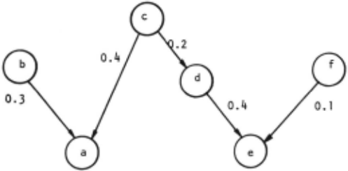
evant to the body temperature can be high, normal, or low. For the sake of discussion, each variable is assumed to have only two possible values (e.g. true or false). The uppercase letter, such as X and X are used to abbreviate x = X and x = X respectively. A simple Bayesian network is shown in Fig. 1.
Both the arcs and nodes in a Bayesian network are quantified by probability functions. The probability func tion of a node with variable x is the a priori probabil ity distribution Pr(x ). The probability function of an arc connecting a node with variable y to a node with variable xis the conditional probability Pr(xly) 1 . The joint dis tribution of the variables can be obtained by multiplying appropriate probability functions together. For example, Pr( abcdef) = Pr( albc )Pr(b )Pr( c )Pr( dlc)Pr( eldf)Pr(f) in Fig. 1.
A permutation of the variables in a Bayesian network can be a composite hypothesis (H) or an evidence (Se) de pending upon whether the variables are observable or not. In general, a composite hypothesis refers to a permutation of a set of quantified variables which include all the vari ables in a Bayesian network except those appears in S ·. However, if this is not the case, such a composite hypothe sis is referred to as local composite hypothesis. For exam ple, there are 6 variables (a, b, c, d, e, f) in Fig. 1; if S. = EF, then ABCD is a composite hypothesis while BCD and DEF are local composite hypotheses 2 .
The inference process of a Bayesian network is based on computing Pr(HISe) to derive the conclusions about the most likely H* (i.e. Max;[Pr(H;JS.)]), or the partial ordering of all H;s, given s ·. When the Bayesian beliefs of all H;s (i.e. Pr(H;IS.)) are computed, a complete partial ordering of all H;s can be generated. In above example, 16 combinations of different values of the variables, a, b, c, d (given Se = EF) have to be considered in order to find a complete partial ordering of all H;s. When k - the number of variables in H;- increases, the number of Bayesian beliefs to be considered correspondingly increases in the order of 2k. It is clear the computational load will soon be a problem when k becomes large. It is unlikely in any application that we need to find a complete partial ordering of the composite hypotheses. However, if we are interested in, for example, the largest four Pr(abcdiEF), applying straightforward approach (i.e. exhaustive evalua tions of all Pr( abcdiEF)) will still require the consideration of all combinations which complexity is in the order of 2k. In next section, we will discuss a set of meta- rules which re duces the computational complexities of deriving a partial ordering of composite hypotheses.
1 Whenever necessary, the conditional joint probability will also be stored; for example, Pr(albc) and Pr(eldf) in Fig. 1 and table 1.
2 Note that a permutation of all variables in a Bayesian network is also a local composite hypothesis by definition. However, this special case is useless to our discussions, thus is excluded from our considerations of local composite hypotheses.
III. Prediction Rule and Conditional Influence
Within the framework of probability theory, Bayesian networks exhibit two properties which lead to a prediction rule for the derivation of a partial ordering of composite hypotheses.
- (i) The composite hypotheses, H;s, of a Bayesian networks are mutually exclusive to each other. Mathematically,
- (ii) The set of all H;, H = U;H;, exhaustively covers all the possible combinations of different values of the variables in a Bayesian network. That is:
Remark: Consider Pr(H; = abcdiEF) discussed above, H1 u 000 u H16 (fork= 4) will lead to AUA, BUB, CUC, D U .fJ. The Bayesian belief of any of these (i.e. Pr(HIS.)) is 1.
Based on the equations (1) and (2), we can derive the following prediction rule:
PRR1 (Prediction rule): Given a partial ordering of the probability of m (out of 2k) mutually exclusive hypotheses Pr(H1IS.) 2: Pr(H2IS.) 2: oo· 2: Pr(Hm IS.) , there is a "'(/ probability that the largest Pr(H;JS.) is within the bound [,8, a] where
H; E {Hm+l . 00 H2t},
C = 1- Pr(H1 U oo . U HmiS.),
a and ,8 are some constants such that Pr(Hm+1 U 000 U H2t IS e) 2: a 2: ,B.
Remark: The proof of above prediction rule (PRR1) can be found in [Sy, 88].
Consider an extreme case that m = 1 and Pr(H1IS.) > 0.5. This implies that the value of C in PRR1 is less than 0.5. If we set ,8 = 0, a = Pr(H2 U 000 U H2t IS.), then PRR1 indicates that H1 is the most likely composite hypothesis with certainty. Next suppose we have m = 3 and Pr(H1IS.) = 0.35 2: Pr(H2IS.) = 0.2 2: Pr(H3IS.) = 0.15. Now Max[Pr(H4 U 000 U H2t IS.)] = C = 0.3. If we set ,8 = 0, a = M ax[Pr(H4 U 000 U H2 k IS.)] 2: Max;,e1,2 ,3[Pr(H;IS.)], we will once again find that Pr(H1IS.) is the most likely composite hypothesis with cer tainty.
From the example shown above, we can see that the rate of reaching a conclusion (about finding either the most likely composite hypothesis or the partial ordering of com posite hypotheses) depends on how and what composite hy potheses are selected for evaluation. That is, if the compos ite hypotheses selected for evaluation have relatively large values of Bayesian beliefs, the faster a conclusion can be reached. Referring to the discussion in Section II and Fig. 1, the Bayesian belief of any arbitrary composite hypothe sis, for example, Pr(abcdiS. = EF), can be rewritten as a joint probability normalized by a priori probability of the variables inS. (Bayes rule). That is:
Each term in the right side (except PrCSe)) can be considered as a probability function for a local composite hypothesis. The change of the Bayesian belief of a per mutation of variables (i.e. abed) depends on the change of the local probabilities (i.e. the terms in the right hand side). The relative changes and the bound of changes are the meta-knowledge for qualitative reasoning and are en coded in terms of "conditional influence".
The probability function for a local composite hypoth esis has a general form Pr( xly1 y2 ... yn) as is observed in (3). Each variable, x or y;, can have two possible values; i.e. X, X or Y;, Y; respectively 3 · Given the value of x, let's say, x = X, we can compare two local probabilities wit~ <!_if ferent values of y;, let's say, Pr(XIYi.Y2) and Prl~IY1Y2) (for n = 2). Suppose Pr(XIY1Y2) ~ ~r_(XIY1Y2), we denote such an inequality by (X IY1 Y2, X IY1 Y2). _8imilarly, (Y11Zt, Y1IZ1) denotes Pr(YdZ1)_ ~ Pr(YdZI), and (Z1,Z1) denotes Pr(ZI) ~ Pr(ZJ). To simplify our dis cussion, we use Y; to represent one permutation o~ t_!le quantified value of y1y2 .. ·Yn· For example, Y1 = Y1Y2, Y2 = Y1Y2, Ys = Yi.Y2, and Y4 = Y1Y2 for n = 2. In ad dition, we use "I" to denote the collection of all (·)s. Using these notations, Conditional influence can be defined as a relation over Ixi as follows:
If there exists (XIY;,XIYj} and (YkiZI,YviZt) such that Yk occurs in Y; and Yv occurs in Yj (for any k f. v), then these two ( ·) s are related to each other under conditional influence relation and the relation is represent ed as an ordered pair shown below 4 :
Referring to the Bayesian network in Fig. 1 and the numer ical values of the probabilistic information shown in table 1, there are 19 such relations. They are:
CI01: ((AIBC,AIBC),(B,B))
CI02: ((AIBC,AIBC),(B,B))
CI03 : ((AlEC, AlEC), ( C, C))
CI04: ((AIBC,AIBC),(C,C))
CI05: ((AIBC,AIBC),(C,C))
CI06: ((AIBC,AIBC),(C,C))
CI07: ((AIB,AIB),(B,B)) CI08: ((AIC,AIC),(C,C)) CI09: ((f>IC,f>IC),(C,C)) cno: ((EIDF,Eif>F),(DIC,f>IC))3 Note that the discussion here can be generalized for variables with multi-values other than binary values.
4 If Yk and Yv have no "parents" in the Bayesian net work, then the relation will be ((XIY;,XIYj),(Yk,Yv)).
Clll: ((EIDF, Elf> F), (DIC, f>IC))
Cll2 : ( (EIDF, Elf> F), (DIC, f>IC)) Cll3: ((EIDF, EIDF), (F, F)) Cll4: ((Eif>F,EIDF),(F,F)) Cll5: ( (EIDF, Elf> F), (DIC, f>IC)) Cll6 : ((EIDF,EIDF), (F,F)) Cll7: ((EID,Eif>),(DIC,f>IC)) Cll8: ((Elf>, EID), (f>IC, DIG)) Cll9: ((EIF,EIF),(F,F))In next section we will show how the conditional influ ence relations are used in qualitative reasoning.
IV. Recognition, Combination, and Propagation Rules
Using the conditional influence relations discussed in Section III, we can examine the qualitative change of the Bayesian belief of a composite hypothesis (i.e. a permuta tion of quantified variables) with respect to the change of the probabilities of local composite hypotheses. For exam ple, when the composite hypothesis accounted for by abed is changed from ABCD to ABCD, CI04 and CI09 indi cate an increase in the probabilities Pr(albe), Pr(dle), and Pr(e), thus the Pr(abediS,).
The selection of composite hypotheses for evaluation during the reasoning process can be based on the condi tional influence relations which induce partitions 5 among the local composite hypotheses. For example, the Bayesian belief of the composite hypothesis ABC f> (given S, = EF) in Fig. 1 can be expressed as below:
There are six terms (excluding Pr(~F)) in the right hand side of above expression. These terms can be parti tioned into 4 classes according to the conditional influence relations. They are:
| Class 1 (according to CI04) : | Pr(AIBC)Pr(C) |
| Class 2 (not exist in CI) : | Pr(B) |
| Class 3 (according to CI09): | Pr(DIC)Pr(C) |
| Class 4 (according to Cll4): | Pr( Elf> F)Pr( F) |
Formally, a class refers to the collection of local com posite hypotheses which achieve local consistency; i.e., the change of the probability value of one variable (due to the change of its quantified value) will lead to the same qualitative change of the overall probability of the class. For example, when the value of the variable e is changed from C to C, the values of both Pr(e) and Pr(albe) will decrease, thus the overall probability Pr( a I be )Pr( e) in class 1 will de crease. Similarly, when the value of a is changed from A to A, the probability Pr(albe) increases, so as Pr(albe)Pr(e).
It is possible to change the value of one variable in one class, which simultaneously leads to the change of the overall probabilities of other classes in an inconsistent way. For example, when the value of dis changed from Jj to D, Pr(EidF) will increase as does the overall probability of class 4. However, this will also cause the decrease of the probability Pr(dic) in class 3, thus causing a decrease in the overall probability of class 3.
5 The partition is not necessarily mutually exclusive.
In order to determine which composite hypotheses sh ould be selected for evaluation, we need to identify those composite hypotheses with which local composite hypothe ses are consistent not only within a class, but also among classes. In the selection of composite hypotheses for evalua tion, three kinds of rules are required in qualitative reason ing. They are (i) the recognition rule, (ii) the combination rule, and (iii) the propagation rule.
Recognition rule - This rule is for class composition. It is used to recognize the pattern(s) of conditional influence existing in a given composite hypothesis and to partition it into classes, or to combine two classes together if the local composite hypotheses of two classes are consistent with one another. The recognition rule used for class composition can be formulated as below:
RR1 (Recognition rule):
(i) If a local composite hypothesis does not exist in any ordered pairs of conditional influence, it is a separate class by itself.
(ii) Otherwise, a class is generated using the composition operation, ffi, defined as below:
where <t:: · » denotes a collection of local composite hy potheses which are consistent to each other in the same class (i.e. local consistency).
Combination rule - This rule is used during the course of reasoning to seek out new hypothesis (i.e. quan tified propositional variable) which can be categorized into a given class. The combination rule is defined through the combination operation 181 described below:
CR1 (Combination rule):
Propagation rule - This rule is for generating con clusion about the potential change of a Bayesian belief due to the change of the probabilities of the partitioned classes. It is used to propagate the conclusions about the combined qualitative changes of the probabilities of two classes; i.e., increase (l), steady (-),decrease(!), or unknown(?). The following table summarizes the qualitative change of the overall probability of a combined class with respect to the change of the probability of each individual class.
| cl \1::', | l - | ? | |
|---|---|---|---|
| l | l | l | ! ? ? |
| - | l | - | ! ? |
| ! | ? | ! | ? |
| ? | ? | ? | ! ? ? |
Qualitative reasoning is envisioned as a process of ap plying the rules described above in a certain sequence for the selection of composite hypotheses for evaluation, and for the generation of conclusions about the qualitative val ues of the Bayesian beliefs of the composite hypotheses. Within the scenario of finding the partial ordering of Pr(H;ISe), the mechanism of reasoning follows as below:
Step 1:
Randomly select a new composite hypothesis for ex amination.
Step 2:
Apply the recognition rule to the composite hypothesis for class partition.
Step 3:
Modify the value of a propositional variable in the com posite hypothesis and re-examine the local consistency of a class using the combination rule.
Step 4:
Apply the propagation rule to generate a conclusion about the overall change of the Bayesian belief of a permu tation of propositional variables.
Step 5:
Re-iterate step 2 to 4 until maximum global consis tency is obtained.
Step 6:
Evaluate the quantitative value of the Bayesian belief of the selected composite hypothesis.
Step 7:
Use prediction and/or heuristic rules to determine whether the conclusion is reached and whether the reason ing process can be terminated.
V. Example
Qualitative reasoning of the Bayesian belief discussed in this paper can be illustrated through the Bayesian net work shown in Fig. 1. The problem is to determine the partial ordering of three most likely composite hypothesis given Se = EF. To start the reasoning process, assume H = ABCD is selected (according to CIOl) for consid eration. The mechanism of qualitative reasoning is shown below: ·
QRl:
Consider CI01, initial setting of abed is H = ABC Jj Apply the recognition rule to H = ABCD
Class 1 (according to CIOl) :
Class 2 (not exist in CI) :
Class 3 (not exist in CI) :
Class 4 (according to C114):
Pr(AIBC)Pr(B)
Pr(C)
Pr(DIC)
Pr(EIDF)Pr(F)
Consider CI02, the value of abed is modified to H = ABC Jj Apply the combination rule to Classes 1 and 2
Class 1 (according to CI02, 03): Pr(AIBC)Pr(B)Pr(C)
Class 2 (according to CI09): Pr(DIC)Pr(C)
Apply the propagation rule to trace the change of H from A.fJC.D to A.fJC.D, we can conclude Pr(ABCDIEF) ~ Pr(ABCDIEF).
Evaluate Pr(ABCDIEF) =? Pr(ABCDIEF) = 0.178.
Mark ABCD, reinvokes the qualitative reasoning pro cess to search another likely composite hypothesis with the same initial consideration; i.e., H = ABCD.
QR2:
Consider CI01, we get H = ABCD as is in QRL
Consider CI15, the value of abed is modified to H = ABCD
Apply the combination rule to classes 3 and 4 shown in QRL
Class 1 (according to CI01) : Pr( AIBC)Pr( B)
Class 2 (not exist in Cl): Pr(C)
Class 3 (based on Cll5, 16): Pr(DIC)Pr(EIDF)Pr(F)
Apply the propagation rule to trace the change of H from ABCD to ABCD, we can conclude Pr(ABCDIEF) ~ Pr(ABCDIEF).
Evaluate Pr(ABCDIEF) * Pr(ABCDIEF) = 0.140.
QR3:
Consider CI04, the initial setting of abed is H = ABCD. Apply the recognition rule to H = ABCD.
Class 1 (according to CI04) :
Class 2 (not exist in Cl) :
Class 3 (according to CI14) :
Pr(AIBC)Pr( C)
Pr(B)
Pr(EIDF)Pr(F)
Evaluate Pr(ABCDIEF) * Pr(ABCDIEF) = 0.159.
Combining the results obtained from QR1, QR2, and QR3, the partial ordering of three most likely composite hypotheses is 6 :
Pr(A.fJCDIEF) ~ Pr(ABCDIEF) ~ Pr(ABCDIEF)
VI. Conclusion
This paper presents a qualitative reasoning approach for the derivation of partial ordering of composite hypothe ses in a Bayesian network. The mechanism of the reason ing process is based on a set of rules which are used to de rive qualitative conclusions about the ordering of the causal relationships of the hypotheses encoded as conditional in fluence relations. This approach features several distinct significances which make it an attractive alternative to be considered for use in probabilistic reasoning. First, the par titions induced by conditional influence permit local rea soning, thus concurrent processing. Second, reasoning in a partitioned class reduces computational complexities, and yet its consistencies between local and global levels are as sured. Third, this approach can be used to infer not only the most likely composite hypothesis, but also the ordering of composite hypotheses. Finally, it is equally important to note that (i) the conclusions generated by qualitative reasoning are usually weaker; e.g., the ordering of the com posite hypotheses are known but not their quantitative val ues, (ii) the efficiency of this approach depe):lds on both the topological structures of a Bayesian network and its prob ability distribution, and (iii) several other approaches are available and equally attractive if our interest is only on the most likely composite hypothesis.
6 A complete partial ordering of Pr( abcdiEF) is shown in table 2.
VI. References
[Cooper, 86] G.F. Cooper," A Diagnostic Method that uses Causal Knowledge and Linear Programming in the Applica tion of Bayes' Formula," Computer Methods and Programs in Biomedicine, Vol. 22, pp. 223-237, 1986.
[Cooper, 87] G.F. Cooper, "Probabilistic Inference Using Belief Networks is NP-hard," Knowledge Systems Labora tory, Stanford University, Memo KSL-87-27, May 1987 (Revised Aug. 1987).
[Pearl, 86] J. Pearl, "FUsion, Propagation, and Structuring in Bayesian Networks," Artificial Intelligence, Vol. 28, pp. 241-288, 1986.
[Pearl, 87] J. Pearl, "Distributed Revision of Composite Beliefs," Artificial Intelligence, Vol. 33, pp. 173-215, 1987. [Rege, 88] A. Rege and A.M. Agogino, "Topological Frame work for Representing and Solving Probabilistic Inference Problems in Expert Systems," IEEE Trans. on Systems, Man, and Cybernetics, May/June 1988, Vol. 18, pp. 402414.
[Sipser, 88] M.F. Sipser, "We still don't know if P = NP", MIT Computer Science Research Symposium, Oct. 1988. [Sy, 88] B.K. Sy, "Qualitative Reasoning of Quantitative Uncertainty in Bayesian Networks," Proc. of the Inter national Computer Science Conj., Hong Kong, December 1988.
[Sy, 89] B.K. Sy, "An Al-based CAD /CAM Approach to Assess Design Methodology of a User-specific Nonvocal Communication Device," Proc. of 15th Northeast Bioengi neering Conf., Boston, March 1989.
| Pr(B) = 0.4 | Pr(C) = 0.65 | Pr(F) = 0.55 | |
| Pr(DIC) = 0.2 | Pr(DIC) = 0.8 | ||
| Pr(AIB) = 0.3 | Pr(AIB) = 0.65 | Pr(AIC) = 0.4 | Pr(AjC) = 0.714 |
| Pr(EID) = 0.4 | Pr(EID) = 0.17 | Pr(EIF) = 0.1 | Pr(EIF) = 0.465 |
| Pr(AIBC) = 0.8 | Pr(AiBC) = 0.6 | Pr(AjBC) = 0.4 | Pr(AjBC) = 0.2 |
| Pr(EjDF) = 0.26 | Pr(EIDF) = 0.14 | Pr(EjDF) = 0.74 | Pr(EjDF) = 0.06 |
| Pr(abcdef) = Pr(ajbc)Pr(b)Pr( c)Pr(djc)Pr( ejdf)Pr(f) | |||
Table 1 : Probabilistic Knowledge of Fig. 1
Pr(A.BCDjEF) ~ Pr(ABCD!EF) ~ Pr(A.BCDjEF) ~ Pr(ABCD!EF) ~ Pr(ABGDjEF) ~ Pr(A.BCDjEF) ~ Pr(ABGDjEF) ~ Pr(ABCDjEF) ~ Pr(ABCD!EF) ~ Pr(A.BCDIEF) ~ Pr(AECDIEF) ~ Pr(A.BCDjEF) ~ Pr(ABCDjEF) ~ Pr(ABCDjEF) ~ Pr(ABCDjEF) ~ Pr(A.BCDjEF)
Table 2: Complete Partial Ordering of Pr(abcdjEF)
@inproceedings{ijcai1989p181,
  title     = {Qualitative Reasoning of Bayesian Belief Using Meta-knowledge},
  author    = {Sy, Bon K.},
  booktitle = {Proceedings of the Eleventh International Joint Conference on
               Artificial Intelligence, {IJCAI-89}},
  publisher = {International Joint Conferences on Artificial Intelligence},
  editor    = {N. S. Sridharan},
  pages     = {1128--1132},
  year      = {1989},
  month     = {8},
  note      = {Commonsense Reasoning},
  url       = {https://ijcai.org/proceedings/1989/181},
}
TY - CPAPER TI - Qualitative Reasoning of Bayesian Belief Using Meta-knowledge AU - Sy, Bon K. T2 - Proceedings of the Eleventh International Joint Conference on Artificial Intelligence, IJCAI-89 PB - International Joint Conferences on Artificial Intelligence PY - 1989 SP - 1128 EP - 1132 UR - https://ijcai.org/proceedings/1989/181 ER -Copied
Machine-readable versions of this paper, for tools and AI agents:





