
Comparative Analysis
Proceedings of the Tenth International Joint Conference on Artificial Intelligence. Reasoning. Pages 959-964.
© 1987 International Joint Conferences on Artificial Intelligence
Abstract
Comparative analysis answers questions about how and why a system will react to perturbations of its parameters. For example, comparative analysis can explain why the period of a spring/block system would increase if the mass of the block were larger. This paper formalizes the problem of comparative analysis and describes a solution technique, differential qualitative analysis; the technique only works if the system can dynamically change perspectives when it compares the values of parameters over intervals. This paper shows how perspectives can be used for comparative analysis, summarizes a soundness proof for the technique, demons·trates incompleteness, describes a working implementation, and presents experimental results .
- Brown J ., de Kleer, J. A Qualitative Physics based on Confluences. Artificial Intelligence, 24, December 1984.
- Doyle J., Steele G. L., de Kleer, J., and G. J. Sussman. Amord: Explicit Control of Reasoning. In Proceed- ings of the Symposium on Artificial Intelligence and Programming Languages, SIGART, Rochester, N.Y., August 1977.
- K. Forbus. Qualitative Process Theory. Artificial In- telligence, 24, December 1984.
- Stevens A., Forbus, K. Using Qualitative Simula- tion to Generate Explanations. Technical Report 4490, Bolt Beranek and Newman Inc, March 1981.
- B. Kuipers. Qualitative Simulation. Artificial Intelli- gence, 29, September 1986.
- D. Weld. Comparative Analysis. AI Memo 951, MIT Artificial Intelligence Laboratory, 1987.
- D. Weld. Explaining Complex Engineered Devices. Technical Report 5489, Bolt Beranek and Newman Inc, November 1983.
- D. Weld. The Use of Aggregation in Qualitative Sim- ulation. Artificial Intelligence, 30(1), October 1986.
- B. Williams. Doing Time: Putting Qualitative Rea- soning on Firmer Ground. In Proceedings of the Na- tional Conference on Artificial Intelligence, pages 105- 112, August 1986.
- B. Williams. Qualitative Analysis of MOS Circuits. Artificial Intelligenc" December 1984.
- Weld
References were extracted automatically from the PDF and may contain errors.
Full text extracted automatically from the PDF; figures, tables and equations may differ. The PDF is the version of record.
1 Introduction
The problem of symbolic analysis of real-world systems is central to many problems in artificial intelligence. In or der to cope with a changing world one must be able to understand its behavior. Recently, considerable empha sis has been put on a specific kind of analysis: qualitative simulation[1,3,10,5,8]. Qualitative simulation seeks to pro duce a description of the behavior of a system over time, often in the form of a tree of histories of the system's qual itatively interesting changes over time [9] .
This paper discusses the problem of comparative anal ysis, in many ways the complement of qualitative simu lation. Whereas qualitative simulation takes a structural description of a system and predicts its behavior, compar ative analysis takes as input this behavior and a perturba tion and outputs a description of how the behavior would change as a result of the pertubation.
For example; given the structural description of a hori zontal, frictionless spring/block system (i.e., Hooke's law), a qualitative simulator would say that the block would first move one direction, stop, then reverse, etc. A description of oscillation would be produced. Comparative analysis,
1 This report describes research done at the Artificial Intelligence Laboratory of the Massachusetts Institute of Technology. Support for the laboratory's Aritificial Intelligence research is provided in part by the Advanced Research Projects Agency of the Department of Defense under Office of Naval Research contract N0014-85-K-0124. Portions of this research were done at Xerox Palo Alto Research Center and at Schlumberger CAS Palo Alto Research.
Comparative Analysis
Daniel S. Weld
MIT Artificial Intelligence Lab Cambridge, MA 02139
on the other hand, should take this description of oscilla tion and evaluate the effects of perturbations. For exam ple, comparative analysis should deduce that if the mass of the block were increased, the period of oscillation would lengthen and explain why (figure 1). In this paper, I de scribe differential qualitative a.nalysis, 2 which solves com parative analysis problems in much the same way as 1. Just as qualitative simulation works without explicit equations for the value of each parameter as a function of time, dif ferential analysis does not need a formula. for the period of oscillation.
Since force is inversely proportional to posi tion, the force on the block will remain the same when the mass is increased. But if the block is heavier, then it won't accelerate as fast. And if it doesn't accelerate as fast, then it will al ways be going slower and so will take longer to complete a full period. 3
Figure 1: Why Period Increases with Mass
1.1 Why is it Interesting?
Comparative analysis is an important component of many artificial intelligence problems including automated design and computer-aided instruction. Suppose a library design for a VLSI pullup circuit has too long a rise time. If the problem solver considers increasing the width of some wire to decrease the rise time, it would like to know the ramifi cations of this modification relative to the initial behavior. Comparative analysis provides this answer, in qualitative terms, as is appropriate for initial design evaluation.
A key subproblem of CAl is the automatic explana tion of the behavior of complex systems. Most AI work in this direction has focussed on techniques for the quali tative simulation of systems [7,4]. Qualitative simulation is an important component of explanation generation, but understanding how systems respond to changes is a useful addition. Explanation generation is the application which most influenced the development of differential qualitative analysis.
2 Differential qualitative analysis was first suggested by Forbus(3, pages 159-161]; section 5 explains the limitations of his approach.
1.2 Perspectives
Differential qualitative analysis [3,6, pages 159-161] is a technique for solving comparative analysis problems in the manner of figure 1. But the differential technique is not as simple as it appears. Consider the first line of the expla nation. What does it mean to say that the force on the block is the same? Clearly the forces aren't equal at all times; since the period is longer in the second case, there are times when the force is zero in the first system yet pos itive in the second system. What's really meant is that in every position occupied by the two blocks the force applied by the spring is the same. In other words, the force doesn't change from the perspective of position.
Although changes in perspective are implicit in ordi nary english text, they must be explicit if a machine is going to generate the explanation. The main contribution of this paper is to show how perspectives can be used to reparameterize quantities in terms of other quantities be sides time. This does more than allow efficient reasoning; differential analysis wouldn't work on systems such as the spring without the ability to shift between perspectives.
2 Notation and General Results
As my formalism is based on that used by Kuipers for QSIM [5], I start out by summarizing his definitions. All compar ative analysis theorems have been proven [6], but are not included in this paper due to length restrictions.
Definition 1 A PARAMETER is a reasonable function of time.
See [5] for the actual definition of reasonable function; the intuition is that of continuity, continuous differentia bility and a finite number of critical points. Parameters are denoted by capital letters. Thus the velocity of an ob ject might be described by the parameter, V, which is a function that maps times to velocities.
Definition 2 Associated with each parameter are a set of LANDMARK VALUES, each is a member of the parameter's range. The landmark values always include (but aren't re stricted to) zero, the values of the parameter at the begin ning and ending times, and the values of the parameter at each of its critical points. A time, t, is a DISTINGUISHED TIME POINT of a parameter P if it is a boundary element of the set of times that P( t) = Pi for some landmark value Pi·
Landmark values are those values considered to be in teresting to the human observer, and the times when these values are reached are of interest too. When a parameter becomes constant for an interval of time, then it will take on a landmark value for infinite number of time points. This is why the definition only considers the boundary times distinguished.
Definition 3 A SYSTEM is a set of parameters that are related with a STRUCTURAL DESCRIPTION that consists of a finite set of qualitative differential equations defined using the following: time differentiation, addition, multiplication, and relation by monotonic functions.
Kuipers' program, QSIM, takes a system and a set of initial values for each of the parameters and produces a set of possible behaviors for the system; the definitions below describe this behavioral output.
2.1 Qualitative Behavior
Definition 4 Let Po < ... < Pk be the landmark values of a parameter P. For any time t define the value of P at . t as:
Define the direction of P at t as:
Define, Qs(P, t), the state of P at t, as the pair:
The qualitative state over the interval between two ad jacent distinguished time points is defined similarly.
Definition 5 For any parameter P, the BEHAVIOR of P is a sequence of states of P:
alternating between states at distinguished time-points, and states on intervals between distinguished time-points.
Recall that a system contains a set of parameters each with its own landmarks and distinguished time points.
Definition 6 The DISTINGUISHED TIME-POINTS of a sys tem are the union of the distinguished time-points of the parameters. Thus the state of a system changes whenever the state of any parameter changes. The BEHAVIOR of a system is thus a sequence of system-states alternating be tween distinguished time-points and intervals.
To perform comparative analysis it is necessary to ab stract away from specific times, since two different systems may have analogous behaviors, but change states at dif ferent times. This is where my formal treatment diverges from that of Kuipers.
Definition 7 When a system changes from one state to any other distinct state, it is ~aid to TRANSITION. Tran sitions only occur at distinguished time-points, and every distinguished time point marks a transition. It will prove useful to be able to refer to these transitions independent of the time at which they occur, thus the sequence of transi tions for a behavior will be denoted by the set hi}· Every behavior also has a TIME FUNCTION, T, which takes tran sitions to the distinguished time-points when they occur.
The intuition is that each 1 marks an event that changes the state of the system. When comparing two behaviors, I match them up event by event and use the time functions to tell whether one system is changing faster or slower than the other.
2.2 Comparing Two Behaviors
To compare two behaviors, they must be distinguishable; I use the hat accent to denote the second behavior. Thus T denotes the time function of the second system, and F(T(/1 )) denotes the second system's value of F at the time of the first transition. I assume that only systems with identical structural descriptions will be compared. For this paper, space considerations necessitate the additional as sumption that behaviors be topologically equal, as defined below.
Definition 8 The behaviors of two systems, S and S, are TOPOLOGICALLY EQUAL if they have the same sequence of transitions, /o, ... , /k, and forall i such that 0 ~ i ~ k,
and forall i such that 0 ~ i < k,
The assumption of topological equality rules out possi bilities like the block failing to make a complete oscillation if its mass was increased too much, but it does allow a certain pliability. If two behaviors are topologically equal, their respective sets of landmarks must share the same or dinal relationships, but the underlying real values for the landmarks can be different.
As shown in [6], this assumption can be relaxed, but even with it, the problem is nontrivial. Consider two oscil lating spring-block systems. Even if the blocks have differ ent mass and the spring constants differ, the two systems have topologically equal behavior. Yet the relative values of parameters such as period of oscillation may be different. This is what comparative analysis must determine.
Before I can explain the techniques for performing dif ferential qualitative analysis, I need to present a notation for describing the desired output. It's easy to compare the values of parameters at transition points:
Definition 9 Given a parameter, F, and a transition/;, define the RELATIVE CHANGE ofF at /i as follows: 4
4 The curious reader may wonder at the use of absolute values in this definition. In [6], I prove that this definition is equivalent to one without absolute values, and explain the advantages of this approach.
For example, if the two spring-block systems were both started with negative displacement and zero velocity (i.e., X< 0 and V = 0), their first transition would occur when X reached zero. This notation allows one to express that the second block is moving slower at the point of transition: V~1 · It is important to distinguish the relative change no tation from statements about values and derivatives. Even though v~l> QVAL(V, T(Tl)) is positive, and qdir(V, 7(11)) is std.
2.3 Comparing Behaviors over Intervals
It turns out to be somewhat more complicated to compare two behaviors over the intervals between transitions. What does it mean to says that one curve is lower than another over an interval? Exactly what points should be compared?
- You can't compare arbitrary points on the two curves, because intuitively it seems that the curve for param eter P(t) =tis lower than that of P(t) = 2t + 1, yet there are some points of P which are higher, e.g., P(4) > P(l).
- You can't use absolute time to link corrresponding points, because P(t) and P(t) might be defined for time intervals of different lengths.
The first line of figure i provides the correct intuition: "If the mass of the block increases, the force on the block is the same." This doesn't mean force is invariant as a function of time-that isn't true. Consider the time when the small bl~ick is at its rest position; the spring applies no force. But since the large block is moving slower, it won't have reached the rest position and so there will be a force applied. What the statement means is that force is invariant as a function of position. For every position that the block occupies, force is equal in the two systems, even though the two blocks occupy the positions at differ ent times. Although parameters are defined as functions of time, they often need to be compared from the perspec tive of other parameters. Here it proved advantageous to consider force as a function of position. Although people understand arguments that leave these changes of variable implicit, the notion must be made precise and explicit if computers are to perform comparative analysis.
Definition 10 Given a parameters F and X , and a tran sition interval ( /;, li+1), Let Fx denote F as a function of X . Let x; = X(T(T;)) and x;+l = X(T(T;+l)). Define the RELATIVE CHANGE ofF over ( /i, li+I) from the PERSPEC TIVE of X as follows:
Two questions remain: when is it possible to use a pa rameter as a perspective, and when is it useful to do so. The first question is easy, but the second will not be addressed until section 3.
Proposition 1 It is possible to use a parameter, X, as a perspective over a transition interval ('y;, 'Yi+t) if and only if the following three conditions hold:
- QDIR(X, T(-y;), T('Yi+t)) =f. std
- XII;
- XII;+I
When these conditions hold, the parameter X is called a COVERING PERSPECTIVE. 5
The intuition behind this proposition is simple. It is only possible to construct Fx when x-t exists; since pa rameters are continuous, X must be strictly monotonic to guarantee invertibility. The last two conditions ensure that Fx and Fx have the same domain so that the universal quantification makes sense. Note the beauty of this result it is computationally easy to check for covering perspec tives.
2.4 Non-Uniqueness
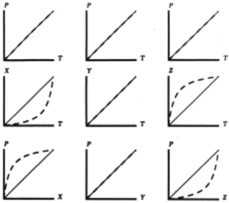
This section shows that parametric comparisons over inter vals are not unique. In other words, just because Pll~,i+I) for a perspective X doesn't mean that there doesn't exist some other perspective Z such that P.ftf;,i+I)'
Although this may seem like a disappointing weakness, it isn't necessarily bad. In fact, it's inevitable. After all, everything is relative to one's perspective. Imagine a ma chine which hourly logs the linearly increasing concentra tion of alcohol in a fermentation tank. It produces the following sequence of measurements: 0.02, 0.04, 0.06, 0.08, etc. But in the identical tank nearby, the logging machine has a defective motor which runs too slowly and delays the measurements. Although the fermentation is proceeding at the same pace in both tanks, the second log will read: 0.03, 0.06, 0.09, 0.12, etc. Thus the plant inspector, who only sees the alcohol-time curve from the perspective of the logging device, might think that second tank was ferment ing more quickly even though the only real change was a slowdown in the speed of the timing motor.
Proposition 2 Given a system with parameters P, X, Y, and Z such that X,Y and Z are covering perspectives over ('Y;,'Yi+t), then it is possible that P.(t~,i+I) and Pllf;,i+I) and PJJ.f;,i+I)'
The example shown in figure 2 illustrates the proof by construction. The thin lines indicate the values of the first system while the dotted lines indicate the value of the. sec ond system. The ·first row shows that from the time per spective the behavior of P doesn't change. The second row shows the relative change of the perspectives. The third row depicts Px, Pr and Pz.
1Spaee coDJideratioDJ preclude an important generalization of per· 1pectivea; .ee [6] for the details.
3 Differential Analysis
This section presents a representative sampling of the in ference rules which have been incorporated as part of CA a. ZETALISP program which solves comparative analysis prob lems using the differential qualitative technique. The rules are presented as theorems since they have been proven sound [6]. As a result, CA is guaranteed to produce only correct answers.
3.1 Duration Rule
This rule is the basis for the very powerful inference: dis tance equals rate times duration. If the rate is slower in the second simulation, then it will take longer to reach the same transition point. Although this may seem obvious, perspectives are required to make precise the notion of 'rate is slower'; this makes it subtle. Note that the parameter X has a double purpose in this theorem: it has V as its time derivative, and it is also the perspective from which V is seen to J,J.. Furthermore, it is unnecessary to explicitly require X to traverse the same distance in the two systems because X is a covering perspective.
Proposition 3 The Duration Rule Let V and X be parameters. 6 Given V = f, X, VJJ.~.i+t)· and X is a covering perspective, then T( 'Yi+t) - T( -y;) > T(-y;+1 )-T('Y;), i.e. the duration of('Y;,/i+t) will increase.
The duration theorem is implemented as the ARK rule shown in figure 3. Note the close correspondence between . the ARK form and the actual theorem statement; this en sures a correct implementation.
It would be nice if one could show that the duration rule was sound if the premise was weakened to have VJJ.r,,i+I) for some arbitrary covering perspective P. Unfortunately, the non-uniqueness theorem shows that this is false.
8 It may be helpful to think of V u velocity, and X u position.
3.2 Derivative Rule
This rule connects parameters which are time derivatives. The intuition is: if a. parameter is II at the sta.rt of an interval, but its derivative is .JJ. over the interval, then the parameter must be .JJ. over the interval. As a.lwa.ys, the need for perspectives complicates the matter. Note the special role of X both as perspective and second integrand of A.
Proposition 4 The Derivative Rule
Let A, V, and X be parameters such that A = ft_v, V = ftX, and X is a covering perspective over ('y;,'Yi+d· Fur thermore let A andV be positive over the interval ('y;, 'Yi+1). If...,V'(t;, and A.JJ.t,i+l)' Then it is true 7 that V.JJ.t.i+l)'
Above I pointed out the special role of X both as per spective and second integrand of A. It is natural to ask if the derivative rule is true for arbitrary perspectives. U n fortunately, it is not [6].
3.3 Self-Reference and Constants
These rules deal with establishing relative change values for perspectives and constants. Although simple, they are quite important. The intuition behind the first is that if the plant manager was foolish enough to try and use the logging devices to log their own speed, he wouldn't get a useful result. Both the normal and slow machines would record that they turned one full revolution during each revolution of the timing motor.
Proposition 5 Self Reference Rule
For any parameter P, if P is a covering perspective over ('y;, 'Yi+t) then Pll~.i+l)'
Frequently a system will contain a few constant param eters ~hose values never change. The following rules are a. simple way to express relationships between constants in the notation of comparative analysis·. The intuition is that since perspectives just scale time, and constants don't change over time, all perspectives agree on the behavior of constants. If there was no fermentation happening in either vat (i.e. the alcohol concentration was constant in both vats), and the concentration of alcohol wa.s higher in vat two, then both logging devices would agree on this even though their timing motors differed.
Proposition 6 Interval Constant Rule
If a parameter K is a constant over ('y;, 'Yi+1), and K'ft; then for all parameters P, if P is a covering perspective over the interval ('y;,/;+1), then K'ft[.,i+l)'
7 The antagonistic effect of the chain rule makes this rule by far the hardest to prove. I owe special thanks to Dave McAllester who suggested a successful approach; see (6] for the details.
3.4 Rules from Qualitative Arithmetic
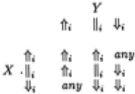
Research in qualitative simulation [1,3,10,5] has developed constraints on derivative values for parameters in ADD, MULT, and monotonic function constraints. For example, if X x Y = Z a.nd the derivatives of X a.nd Y are posi tive, then Z must ha.ve positive derivative as well. These rules ca.n be generalized to include relative change values at transition points and over intervals. Here, I present just the rule for an MULT constraint at a transition point.
Proposition 7 Multiplication Rule
If X, Y, and Z are parameters which are related by the con straint, Z = MULT(X, Y), then the following table displays the possible relative change values for Z at a transition point:
4 Evaluation
To test this theory a program, CA, has been written in ZE TALISP on a. Symbolics lisp machine. When a user selects an example, CA runs QSIM [5] on the example to produce a set of qualitative behaviors for the example. The user se lects a. behavior a.nd a.lso a set of perturbations in the form of initial relative change values for the independent param eters. CA translates the QSIM behavior and perturbations into ARK 8 assertions. At this point ARK forward chains using the rules of the last section. Figure 3 shows the en coding of proposition 3 as an ARK rule. The simplicity of the transformation leads to confidence in the correctness of the implementation. And the fact that most rules get used in each explanation, establishes their utility.
(=> (a.nd (d/dt ?x ?v)
(rc ?v ?int ?c ?x)
; ?vis derivative
; ?c is rel. change of ?v
(opposite-rc ?c ?oc)) ; from perspective of ?x
(duration ?int ?oc) ; if ?cis'(}', ?oc is .JJ.
DURATION-RULE)
; ?int is transition interval
Figure 3: Propositions are Encoded into ARK Rules
4.1 Differentia.! Analysis Usually Works
Since ARK maintains justifications for all its assertions, it is possible to generate explanations for CA's conclusions. Consider the spring/block example. The system is defined in terms of four independent parameters: spring constant [(, mass M, position X, and velocity V and two others:
8 ARK is a 'clean' descendent of AMORD [2] implemented by Howie Shrobe and others.
acceleration A, and force F obeying the following equa tions: A = f, V, V = f,X, F = MULT(M,A), and F = MULT(K, X) . In addition M and ]( are constant. The initial conditions are specified as follows : M(O) > 0, I<(O) < 0, V(O) = 0, and X(O) = xo < 0.
Since energy conservation is not made explicit in the equations, QSIM produces three possible behaviors for this system: stable oscillation, decaying oscillation, and ex panding oscillation. Although comparative analysis could be done on any of the behaviors, I assume in this exam ple that the user selects the (correct) interpretation: stable oscillation.
Assuming we are interested in the system's behavior when the block's mass is increased, we must select the ini tial relative change values for the independent parameters: Mi)"0 , Kll 0 , Vll 0 , and Xllo·
Given this information, CA correctly deduces that the block will take longer to reach the rest position (X = 0) from its original negative stretched position. Figure 4 shows the explanation for this fact that CA generates by throwing away all perspective information once computa tion is finished. I have annotated the explanation with the names of rules used in each step.
| Assuming M is increased: | |
|---|---|
| X doesn't change and | {self-reference) |
| K doesn't change and | {interval constant) |
| F equals K times X | |
| So F doesn't change. | {multiplication) |
| and | |
| M increases and | {interval constant) |
| F equals M times A | |
| So A decreases. | (multiplication) |
| So V decreases. | (derivative) |
| So the time duration increases. | {duration) |
At present CA has been tested for several different per turbations on over a dozen examples [6]. While it has never produced an incorrect answer, CA doesn't always produce a result.
4.2 Differential Analysis is Incomplete
There are three factors that can cause differential qualita tive analysis to fail to predict all of the relative changes in a perturbed system: nonexistence of an answer, ambiguity resulting from the qualitative arithmetic, and the nonexis tence of a useful perspective.
4.2.1 No Answer Possible
Some questions simply don't contain enough information. For example: "What would happen to the period of oscil lation, if the mass of the block was heavier and the spring was more stiff?" Noone can answer this question, because there is no answer. The increased mass tends to increase the period, but the increased sping constant tends to de crease it. Thus the duration might increase, decrease or remain unchanged.
4.2.2 Ambiguity
Since differential analysis uses the same weak qualitative arithmetic utilized by other forms of qualitative reasoning, it should not be surprising that ambiguity causes a prob lem here as well. Consider the spring/block system of the last section. Differential analysis correctly predicts that the block will take longer to reach the first transition, the block's rest position. But the period of oscillation requires four transitions: starting from a negative initial position, X transitions to zero, then to a positive maximum, then to zero, and finally to its original position. Because of ambigu ity in the extreme positions of X , differential analysis can make no prediction about duration of these last three tran sition intervals. Why is this? Because of the qualitative arithmetic, it is impossible to show that Xll 2 , i.e., that X sweeps out the same distance when the mass is increased. As a result, X is not known to be a covering perspective so the derivative and duration rules can not be used. Thus there is no way to determine the relative change value for the whole period.
If the structural description of the spring is augmented with equations describing conservation of energy, 9 CA can deduce that since potential energy is equal to force times distance, increasing the block's mass leaves total energy unchanged. This allows it to recognize X as a covering perspective and deduce that the duration increases for each of the period's four transition intervals.
4.2.3 No Useful Perspective
Other questions are even more difficult to answer: "What would happen to the period of oscillation if the initial dis placement is increased?" Since people have trouble with this question, it should not be surprising that differential analysis cannot answer the question either. In fact, the an swer is "period does not change", but the only way to show this is to solve the differential equation for an equation for period and notice that it is independent of amplitude. The difficulty is rooted in the fact that no useful perspective ex ists to provide a handle on the problem. There is no system parameter P such that Vll[o,t)· Clearly X won't work as. a perspective, since it doesn t sweep out the same range m the two cases. In fact, it is easy to prove that no artifical perspective could satisfy the equation [6].
5 Related Work
Despite its importance, little work has been ?one o~ co~ parative analysis. Forbus discussed differenttal quahtattve analysis (3, pages 159-161], but attempted no implementa tion. He defined quantities q1 greater than q2 over an in terval, i, if for all instants in the interval, q1 > q2 measured at that instant. Unfortunately, this definition has several problems. Since the quantification is over a single interval of time, it is impossible to make comparisons of systems whose time behavior changes as a result of a perturbation. Thus his attempt to formalize "distance equals rate times duration" in predicate calculus is useless. Rates can only be compared if the duration of an interval is unchanged!
9 AB Kuipers did to make QSIM eliminate physically. im~ossible behaviors of the spring leaving only the correct stable oscillatiOn pre diction (5].
But even if the quantification was ok, Forbus' compari son is almost never a useful one to make. In the spring/block case, for example, it simply isn't the case that the heavy block is always moving slower than the small-block; the periods get out of phase. The key to solving these prob lems is in the use of perspectives, discussed in this paper. The comparison on velocity (necessary to predict that the period lengthens) is valid only from the perspective of po sition.
Other fields of study address related problems. Engi neering sensitivity analysis considers quantitative answers to comparative analysis questions. However, sensitivity analysis does not generate explanations, and it could not solve the spring/block problem without an explicit equa tion for period.
6 Conclusions and Future Work
This paper has discussed the problem of comparative analy sis and emphasized the differential solution technique. The major advance over previous work is definition of interval comparisons using perspectives. This has allowed a fast im plementation of the technique, precise formalization, and a proof of soundness.
But differential qualitative analysis is just one way to solve comparative analysis problems. Another technique is EXAGGERATION which solves the original spring/block problem with following explanation:
"If the mass were infinit~hen the block wouldn't move, so the period would be inflnite. · Thus, if you increase the mass by only a little bit, then the duration of the period would increase a bit as well."
Exaggeration is a kind of asymptotic analysis-the per turbation is taken to the limit to make the effect more easily visible. Exaggeration is common in intuitive descriptions of physical behavior and appears quite powerful. As the example shows it often results in a concise explanation.
But exaggeration is also tricky. It works only when the system responds monotonically to perturbations. Fur thermore, it requires non-standard analysis to reason about infinity; it's quite easy to concoct a plausible exaggerated argument which is faulty. A careful formalization of the technique is the topic of current research.
Perhaps the greatest liability of differential qualitative analysis is its incompleteness. Although exaggeration is likely to be incomplete as well, early results suggest that it will work in cases when differential analysis fails. A program which uses both techniques could prove exceptionally powerful.
ACKNOWLEDGEMENTS
This work was greatly influenced by discussions with too many people to list here, but Jeff Shrager, David McAllester, Tomas Lozano-Perez, Ben Kuipers, Glenn Kramer, Pat Hayes, Johan de Kleer, and Ernie Davis were especially helpful. Brian Williams, Mark Shirley, Jerry Roylance, Ken Forbus, and Randy Davis provided helpful comments on early drafts.
@inproceedings{ijcai1987p198,
  title     = {Comparative Analysis},
  author    = {Weld, Daniel S.},
  booktitle = {Proceedings of the Tenth International Joint Conference on
               Artificial Intelligence, {IJCAI-87}},
  publisher = {International Joint Conferences on Artificial Intelligence},
  editor    = {John McDermott},
  pages     = {959--964},
  year      = {1987},
  note      = {Reasoning},
  url       = {https://ijcai.org/proceedings/1987/198},
}
TY - CPAPER TI - Comparative Analysis AU - Weld, Daniel S. T2 - Proceedings of the Tenth International Joint Conference on Artificial Intelligence, IJCAI-87 PB - International Joint Conferences on Artificial Intelligence PY - 1987 SP - 959 EP - 964 UR - https://ijcai.org/proceedings/1987/198 ER -Copied
Machine-readable versions of this paper, for tools and AI agents:





