
An Optimal Scale for Edge Detection
Proceedings of the Tenth International Joint Conference on Artificial Intelligence. Perception. Pages 745-747.
© 1987 International Joint Conferences on Artificial Intelligence
Abstract
Many problems in earl y vision are ill posed 1 . Edge detection is a typical example. This paper applies regularization techniques to the problem of edge detection. We derive an optimal filter for edge detection with a size controlled by .the regularization parameter A and compare it to the Gaussian filter. A formula relating the signal-to-noise ratio to the parameter A is derived from regularization analysis, showing that the scale of the filter is a function of the signal-to-noise ratio. We also discuss the method of Generalized Cross Validation for obtaining the optimal filter scale. Finally, we use our framework to explain two perceptual phenomena: coarsely quantized images becoming recognizable by either blurring or adding noise.
- Tikhonov, A.N. "Solution of Incorrectly Formulated Problems and the Regularization Method," Soviet Math. Dokl. 4, 1035-1038, 1963.
- Poggio, T. and Voorhees, H. and Yuille, A. "A Regu- larized Solution to Edge Detection," Artificial Intelli- gence Lab. Memo, No. 833, MIT, Cambridge, MA, 1985.
- Poggio, T. and Torre, V. "Ill-Posed Problems and Reg- ularization Analysis in Early Vision," Artificial Intel- ligence Lab. Memo, No. 773, MIT, Cambridge, MA, 1984.
- Torre, V. and Poggio, T . "On Edge Detection," Arti- ficial Intelligence Lab. Memo, No. 768, MIT, Cam- bridge, MA, 1984.
- Morrone, M.C. and Burr, D.C. and Ross, J. "Added Noise Restores Recognizability of Coarse Quantized Images," Nature, Vol. 305, 15 Sept. 1983.
- Harmon, L.D. and Julesz, B. Science 180, 1194-1197, 1973.
- Canny, J.F. "Finding Edges and Lines in Images," Ar- tificial Intelligence Lab. Technical Report No. 720, MIT, Cambridge, MA, 1983.
- Wahba, G. "Ill Posed Problems," Technical Report No. 595, 1980.
- Reinsh, C.H. "Smoothing by Spline Functions," Numer. Math., 10, 177-183, 1967.
- Voorhees, H. "Computing Texture Boudaries," S.M. Thesis, MIT, Cambridge, MA, 1987 (in preparation).
- Wilson, H.R. and Bergen, J.R. "A Four Mechanism Model for Threshold Spatial Vision," ViJion Re~earch 19, 19-32, 1979.
- Terzopoulos, D. "Computing Visible-Surface Repre- sentations," Artificial Intelligence Lab. Memo, No. 833, MIT, Cambridge, MA, 1984.
- Marroquin, J . "Probabilistic Solution of Inverse Prob- lems," Artificial Intelligence Lab. Technical Report No. 860, MIT, Cambridge, MA, 1985.
References were extracted automatically from the PDF and may contain errors.
Full text extracted automatically from the PDF; figures, tables and equations may differ. The PDF is the version of record.
1. Introduction
If edge detection is considered as a problem of numerical differentiation, the first step is to regularize it. Standard regularization techniques suggest the use of Gaussian-like filters before differentiation 2 · 4 · In this paper, we address the important issue of how to estimate the optimal scale of the filter, that is, the amount of smoothing required by the given image data.
2. Framework for Edge Detection
Regularization Techniques for Ill-Posed Problems A problem
for which the class S of solutions z , given A and u, is not compact (changes on the right-hand side of the equation can take u outside the set AS) is called ill-posed. The approach suggested by Tikhonov 1 to deal with ill-posed problems is to construct approximate solutions of equation (2.1) that are stable under small changes in the data u . If the right-hand side of equation (2.1) is known only ap proximately, we have u(x,y) = ur(x,y) + v(x,y), where v(x, y) is noise. Then,
AN OPTIMAL SCALE FOR EDGE DETECTION
Davi Geiger and Tomaso Poggio
Massachusetts Institute of Technology Artificial Intelligence Laboratory
where
and k(w,v) is the Fourier transform of k(x,y). It would seem natural to take the solution of equation (2.1) as being
since ur(w,v) = k(w,v)zr(w,v). However, this function may not exist since the last integral may diverge. Fur thermore, even if this ratio does have an inverse Fourier transform, the deviation from zero (in the C-or L2-metric) can be arbitrarily large, and, thus we cannot think of the exact solution of equation (2.1) as an approximate solution of the equation with approximate right-hand side.
Finding edges in an image is in general an ill-posed problem 4 , since it involves taking an appropriate deriva tive of noisy data (notice that we do not specify which derivative operator should be used: it may be a direc tional derivative 4 or any other desirable differential oper ator). The differentiation of u( x) is ill-posed, since it can be viewed as a solution of equation 2.1 for the operator A of the form
where h( x) is the step function. As described by Rheinsch 9 and by Poggio and Torre 3 , this problem can be regularized by smoothing the data before taking derivatives. The idea is to consider the regularized solution z to equation (2.1), with A being the imaging operator, such that z is suffi ciently well-behaved for numerical differentiation.
To approximate a solution of equation (2.1) one takes the solution of a different problem, that of minimizing the functional given by,
that is close to the solution of the original problem for small values of the error in the data. Tikhonov 1 proved that for the case of one dimensional image data. Here u(x, y) is the image data, A is the regularization parameter, A is in our special case a convolution operator and n[z) is the stabilizing operator. We will be considering the special case where
The Fourier transform of(~+~ )PI 2 z is M(w, v)z(w, v), where M(w, v) = (w2 +v2)". The order of the derivative in n[z], controlled by the parameter p, should be high enough to ensure the appropriate degree of differentiability in z required by the desired derivative operation that has to be performed next.
It should be pointed out that, whereas the original problem (2.1) does not have the property of stability, the problem of minimizing the functional M >. [ z, u) is stable under small changes in the right-hand side u. This stability has been attained by narrowing the class of possible solutions by introducing the stabilizing functional n[z).
3. The Optimal Filter
Using Parseval's theorem, we can rewrite equation (2.3) as
The associated Euler-Lagrange equation is
For the special case where p = 2 (stabilize with Lapla cian) and the operator A given by (2.2) and k(w, v) = e-b("' 2 + 112 )/2, we obtain the regularized solution
This corresponds, in the Fourier domain, to filtering the input data with
The case b=O.O (degree)l gives the PVY filter 2. For b = 0.0 the filter is not smooth enough to ensure differ entiability with a second order differential operator such as the Laplacian and a higher order stabilizer is needed 2 . For b > 0 this problem disappears however. The term k(w, v) approximates the modulation transfer function of the imaging device. For the human eye it has bandwith w=60 ( degree)- 1 , implying that b=0.2216 (degree )2. The filter is plotted (b=0.2216) in the space domain for differ ent values of A (figure 1), which controls the size of the filter.
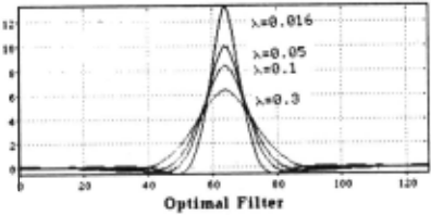
In order to compare the optimal filter with the Gaus sian filter, we have to use some measure for the filter's size. A possible criterion is the frequency at which the amplitude drol:>s to half of its maximun value. This gives _,2""2 -ho12 Gaussian:l. = e~ and optimal-filter:!= _: 2 · ·. ~ e w·+~""'·
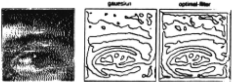
4 -H·;·>t Therefore A = fnie · . Another criterion is to chose filters that have the same width in their (appropriate) derivative. An example is given in figure 3 where the derivative operator is the Laplacian; both filters give very similar zero-crossings.
4. The Optimal Scale
In order to find the optimal scale we vary A to obtain the closest solution to the true solution. More precisely, we minimize
where E{.} is the expectation value operator, S(w, v) is the spectral density (power spectrum) of zr(x, y) and N(w, v) is the spectral density of v(x, y), assuming that v(x, y) is wide sense stationary. In practice, it is a good approxima tion to assume white noise N(w, v) = N 0 and the asymp totic value
For c = 2, we obtain A = ~ and for c = 3, A is the solution of
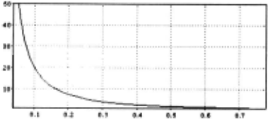
For the case b = 0.0 (the PVY filter) we get A = (5/7) t(-~':· )l . : A graph of signal-to-noise ratio versus .A for b = 0.2216 (degree) 2 is plotted in figure 2. Thus the optimal size of the filter can be obtained directly from an estimate of the signal-to-noise ratio for any given image.
5. Noise Estimation
To estimate the noise we use a technique ,developed by Voorhees 10 . First, the gradient of the image is computed. A Rayleigh distribution is then fitted to the histogram of the norm of the gradient and the noise parameters are es timated. The signal power is obtained from the standard deviation of the histogram of the image. With this method the program estimates the signal-to-noise ratio from the image data. This ratio gives the parameter >. from rela tions such as equation 4.1. The results are shown in figures 3 and 4.
Figure 9. Zero-cro.9sing" wing Gau.9sian filter and optimal-filter with the .9ame width for the .9econd-derivative
6. Two Perceptual Phenomena
6.1. Coarse quantized images can be better recognized when noise is added
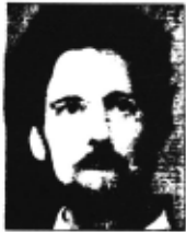
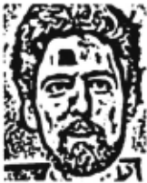
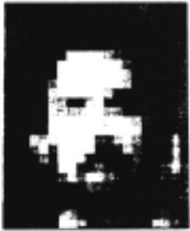
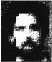
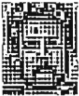
We first discuss the perceptual phenomena of improved recognizability of coarse quantized images when noise is added 5 . Consider the image of figure 4a with 320 by 384 pixels. A coarsely quantized version of it is shown in figure 4c. The optimal filter for figure 4c, estimated as explained above, turns out to have a small scale of ~ 2.0 pixels cor responding to very low noise S 0 / N 0 = 100.0. The sign of the zero-crossings (figure 4d) do not easily reveal a face. Gaussian white noise with standard deviation 70 is the added to figure 4c (see figure 4e), making recognition eas ier. Estimation of the optimal scale gives now a width of ~ 6.5 pixels. The corresponding zero-crossing contours reveal the face in a much better way. These results may shed some light on what the visual system may be do ing. Harmon and Julesz 6 claim that for the quantized image "high frequencies introduced by quantized blocking mask the lower spatial frequencies which convey informa tion about the face, preventing recognition".
::J. Figure 4. a,b) Image of a face and sign of the zero-crossings (szc) using Laplacian operator. c,d) Quantized image and .9ZC with u = 2.0 pixels. e,J) White noise, standard devia tion of 70 units, was added to the quantized image. Now .9ZC is u = 6.5 pixels.
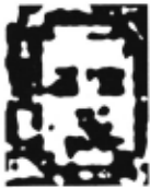
In our framework two process determine recognizability of the face. The first process consists of the estimation of the signal-to-noise ratio (S 0 /N 0 ). The second step is to use So/ N0 to set the optimal >. for then computing an appro priate derivative and corresponding "edges". In the case of the quantized image the ratio So/ No is large. >. is then small, which implies that a large bandwidth channel (in the spatial-frequency domain) is selected. The zero cross ings for this channels do not easily allow face recognition because they mostly capture the box outlines. For noisy quantized images the ratio So/ N0 is small and correspond ingly >. is large. This imply a filter with small bandwidth. In this case the small bandwidth filter suppresses the noise and, as a side effect, also the high frequency outlines of the boxes.
This explanation is not in contrast with the one given by Canny 7 or by Morrone, Burr and Ross when they claim "that added noise (more high frequencies) destroys the propensity to organize the image according to its spurious high-frequency structure, ... ", but is more precise.
6.2. Improved recognizability of coarse quantized images by blurring
Blurring coarsely quantized images also improve recognition 6 · The explanation for this second perceptual phenomena is natural in our model. Blurring is equivalent to using an effectively larger filter for edge detection. This has the effect of suppressing the spurious high frequency edges in troduced by coarse quantization. ·
7. The Method of Generalized Cross Validation and Regularization
When So/No cannot be directly estimated, it is natural to consider the method of Generalized Cross Validation ( GCV) 8 . The GCV method states that the optimal value of >. , can be obtained by minimizing the functional (here in one dimension)
where wk(>.) = (1- au,(>.))/(1- ~ L:j=o ajj(>.)) and
Assuming the filter to be Gaussian-like, using the optimal filter would be computationally more expensive, equation 7.3 reduces to
The method is computationally expensive but intrinsically parallel. We have implemented it on Connection Machine. We tested this method on different images including the ones in figure 4 with various amounts of noise. The im portant result was the consistence of the GCV with the results obtained by a method described earlier. Slices of the image 80 pixels require 20 miliseconds for computing V(u) . Using Newton's method to find the minimun, the algorithm converges after 10 interations of V( u ). There fore the GCV method takes in this case 0.2 seconds to find the optimal u .
8. Conclusion
We have derived rigorously the optimal way of filtering im ages prior to numerical differentiation. We also obtained the precise relation between the scale of the ffiter >. and the signal-to-noise ratio of the image. Some biological im plications were also considered. In particular we suggested that humans can estimate the signal-to-noise ratio in the image from which the scale >. is computed. Only channels channels with the appropriate spatial-frequency band
·Notice that blurring the quantized noisy image has the effect of increasing the estimate of signal-to-noise ratio, thereby re ducing u2 to a value close to the one obtained for the quan tized image.
- are then used, the others being inhibited. In this frame work it is possible to understand the perceptual phenom ena of improved recognizability of coarsely quantized im age when noise is added. When the signal-to-noise ratio is large, the estimated >. is small and the associated zero crossings do not provide good information for recognition. When So/ No is smaller, the estimated>. is larger: the zero crossings provide then a better information for recognizing the face in th~.image . When the signal-to-noise ratio can not be estimated,it is possible to use the method of Cross Validation for estimating the optimal >..
Acknowledgments: We are grateful to A. Yuille for many discussions (with D.G.). Thanks to E. Gamble, M. Gen nert, and H. Voorhees who were always helpful.
@inproceedings{ijcai1987p150,
  title     = {An Optimal Scale for Edge Detection},
  author    = {Geiger, Davi and Poggio, Tomaso A.},
  booktitle = {Proceedings of the Tenth International Joint Conference on
               Artificial Intelligence, {IJCAI-87}},
  publisher = {International Joint Conferences on Artificial Intelligence},
  editor    = {John McDermott},
  pages     = {745--747},
  year      = {1987},
  note      = {Perception},
  url       = {https://ijcai.org/proceedings/1987/150},
}
TY - CPAPER TI - An Optimal Scale for Edge Detection AU - Geiger, Davi AU - Poggio, Tomaso A. T2 - Proceedings of the Tenth International Joint Conference on Artificial Intelligence, IJCAI-87 PB - International Joint Conferences on Artificial Intelligence PY - 1987 SP - 745 EP - 747 UR - https://ijcai.org/proceedings/1987/150 ER -Copied
Machine-readable versions of this paper, for tools and AI agents:





