A New Sense for Depth of Field

A NEW SENSE FOR DEPTH OF FJELD

Alex P . Pentland

Art ificial Intelligence Center, SRI International 333 Ravenswood Ave, Menlo Park, CA 94025

and

Center for the Study of Language and Information Stanford University, Stanford CA 94038

In this paper we report the finding that this gradient of focus in­ herent in biological and most other optical systems is a useful source of depth information, prove that these focal gradients may be used to recover a depth map (i .e., distances between viewer and points in the scene) by means of a few, simple transformations of the image, and that with additional computation the reliability of this depth information may be internally checked. This source of depth information (which differs markedly from that used .in automatic focusing methods) has not prev iously been described in the human vision literature, and we have been unable to find any investigation of it in the somewhat more scattered machine vision literature. The performance of a practical technique has been demonstrated on realistic imagery, and an inexpen· sive, real-time version of the algorithm is described. Finally, we report experiments showing that people make significant use of this depth in­ formation.

This novel method of obtaining a depth map is important be­ cause there is currently no passive sensing method for obtaining depth information that is simultaneously fast enough, reliable enough, and produces a sufficient ly dense depth map to support the requirements of a robot moving in a complex environment . Stereopsis, despite huge investment , remains computationally intensive and prone to severe er· rors, the use of motion information is still in an experimental stage, and autofocus schemes can measure depth at only one point at a time. We believe that this research, therefore, will prove a signiflcant ad­ vance in solving the problern of real-time acquisition of reliable depth maps without the limitations inherent in active scannen (e.g., Iaser rangefinders).

II. THE FOCAL GRADIENT

Most biological Jens systems are exactly focused· at only one dis­ tance along each radius from the Jens into the scene. Tbe locue or exactly focused points forms a doubly curved, approxirnately epberical surface in three-dimensional space. Only when objecte in the ecene in· tersect this surface is their image exactly in focue; objecte diltant from this surface of exact focus are blurred, an elfect familiar to pbotoa· raphers as depth of field.

The amount of defocus or blurring depends eolely on the distance to the surface of exact focus and the characteristice of tbe Jene eyetem; as the distance between the imaged point and the surface of exact focue increases, the imaged objects become progressively more derocueed. lf we could measure the amount of blurring at a given point in tbe image, therefore, it seems possible that we could uee our knowledae of the parameters of the Jens system to compute tbe distance to tbe corresponding point in the scene.

· "Exact focus" is taken here to mean "has the minimum variance point spread function," the phrase "measurement of rocus" is taken to mean "characterize the point spread function ."

ABSTRACT

One of the major unsolved problems in designing an autonomous agent jrobotj that must function in a complex, moving environment is obtain ing reliable, real-time depth information, preferahly without the limitations of active scanners. Stereo remains computat ionally in­ tensive and prone to severe errors, the use of motion information is still quite experimental, and autofocus schemes can measure depth at only one point at a t ime. We examine a novel source or depth informa­ tion: focal gradients result ing from the limited depth or fleld inherent in most optical systems. We prove that this source of information can be used to make reliable depth maps of useful accuracy with relatively minimal computation. Experiments with realistic imagery show that measu rement or these optical gradients can potentially provide depth information roughly comparable to stereo disparity or motion paral­ lax, while avoiding image-to-image matehing problems. A potentially real-time version of this algorithm is described.

I. INTRODUCTION

Our subjective impression is that we view our surroundings in sharp, clear focus. This impression is reinforced by the virtually univer­ sal photographic tradition ·· to make images that are everywhere in focus, i.e., that have in fi nite depth of field . Unfortunately, both this photographic t radition and our feeling of a sharply focused world seems to have Iead vision researchers - in both human and machine vision - to largely ignore the ract that in biologicalsystems the images that fall on the retina are typically quite badly focused everywhere except wi thin tbe centrat fovea j1 ,2j. There is a gradient of focus , rauging from nearly perfect focus at the point of regard to almost complete blur at points on distaut objects.

lt is puzz ling that biological visual systems first employ an optical system that produces a degraded image, and then go to great lengths to undo t.his blurri ng and present us with a subjective impression of sharp focus. This is espec ially peculiar because it is just as easy to start out wi th everyth ing in perfect focus. Why, tben, does Nature prefer to employ a Jens system in which most of the image is blurred?

· This research was made possible in part by a grant from the Systems Development Foundation, and by a grant from the National Science Foundation, Grant No. DCR-83-12766, and by Defense Advanced

Research Projects Agency contract no. MDA 903-83-C-0027

·· A practice established in !arge part by Anse! Adams and others in

the famous "f/64 Club"

The distance D to an imaged point is related to the parameters or the Jens system and the amount or defocus by the rollowing equation, which is developed in the appendix.

where v0 is the distance between the Jens and the image plane (e.g., the film location in a camera), f the r-number or the Jens system, F the focal length or the Jens system, and u the spatial constant or the point spread runction (i.e., the radius or the imaged point's "blur circle") which describes how an image point is blurred by the imaging optics. The point spread function may be usefully approximated by a two-dimensional Gaussian G(r, u) with a spatial conatant u and radial distance r. The validity or using a Gaussian to deacribe the point apread runction is discussed in the appendix.

In most situations, the only unknown on the right-hand aide or Equation (1) is U, the point spread runction's spatial parameter. Thus, we can use Equation (1) to solve for absolute distance given only that we can measure u, i.e., tbe amount or blur at a particular image point.

Measurement or (! presents a problem, however, for the image data is the result or both the characteristics or the scene and tboae or tbe Jens system. To disentangle theae factors, we can either Iook for places in the image with known characteristics (e.g., aharp edr;es), or we can observe wbat happens when we cbange some aspect or tbe Jens system. In the following discussion both or these two r;eneral strategies for measurement or (! are described: the use or sharp edr;es, and comparison across different aperture settinga. Both approachea require only one view or the scene.

A. Uslng Sharp Dlscontlnultlea

Image data are determined both by scene characteristics and the properties or the Jens system, e.g., how rast image intenaity chanr;es depends upon both how scene radiance changes and tbe diameter or the blur circle. Ir we are to measure blur circle, therefore, we muat already know the scenes' contribution to the imar;e. At edr;es - sharp discontinuities in the image rormation process - the rate or chanae we observe in the image is due primarily to the point apread function; because we can often recognize sharp discontinuities with some dearee of confidence j3,4 j we can use image d,ata surroundin& tbem to deter­ mine the focus. These Observations Iead to the rollowin& &eherne ror recovering the viewer-to-scene · distance at pointa of discontinuity.

Mathematica/ Details. To calculate the apatial conatant of tbe point spread function we require a measure or the rate at which imaae intensity is changing; the wide-apread use or zero-crossinas or the Laplacian to find edges j5j sugr;esta using slope of the Laplaci&D acrou the zero-crossing as a measure of rate or change.

Consider a vertical step edae in the image of maanitude 6 at posi­ tion xo. In this case the valuea C(x, y) resultin& from the convolution of image intensities I(x , y) with the Laplacian of a Gausaian V2G(r, 11) (as in j51) have the form

where G(x- x0 , q) is a one-dimensional Gausaian centered at point :~:0 , and q is the spatial constant of the point spread function at that point in the image. For such an edge the slope or the function C(z, y) at the point or the zero-crossing is equal to the maximum rate of chanae in image intensity, and so we can uae it to estimate <1.

*When the discontinuity is in depth , as at an occludin& contour, tbe distance measured is to the nearer side or the diacontinuity .

An estimate or <T can be rormed as follows :

where x, y and 6 are as before, and ror convenience :~:0 is taken to be zero. Taking the absolute value and then the natural log, we ftnd

We can formulate Equation (4) as

Ir we interpret Equation (5) as a linear regre111ion in z2 we can tben obtain a maximum-likelihood estimate or the constantl A and B,

wbere and thus obtain u. The solution of this linear regression is

where% is Lhe mean of the x;, and Cis the mean of the Ct. From A in Equation (6) we can obtain the following estimate of the value of the spatial constant u:

Having estimated u we can now use Equation (I) to find the distance to the imaged point; note that there are two solutions, one corresponding to a point in front of the locus of exact focus, the other corresponding to a point behind it . This ambiguity is generally unimportant because we can usually arrange things so that the surface of exact focus is nearer to the sensor than any of the objects in the field of view.

B. Compariaon Acroaa DlfrerlniJ Aperturea

The limiting factor in the previous method is the requirement that we must know the scene characteristics before we can measure the focus; this restricts the applicability of the method to special points such as step discontinuities. Ir, however, we bad two images of exactly the same scene, but with different depth of field , we could factor out the contribution of the scene to the two images (as the contribution is the same ), and measure the focus directly .

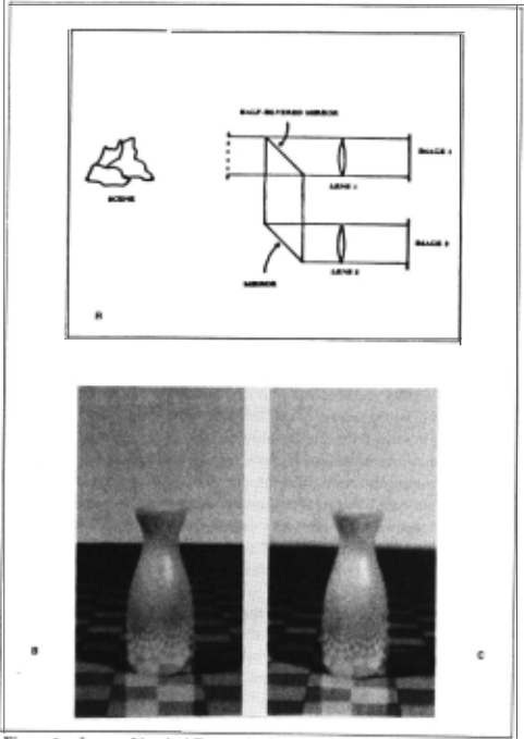
Figure I shows one method of taking a single view of the scene and producing two images that are identical except for aperture size and therefore depth or field . This Jenssystem uses a half-silvered mirror (or comparable contrivance) to split the original image into two identical images, which are then directed through Jens systems with dilrerent aperture size. Because change in aperture does not alrect the position of image features, the result is two images that are identical except" for their focal gradient ( amount of depth of field), and so there is no difficu lty in matehing points in one image to points in the other. Figures I (b) and (c) show a pair of such images. Alternatively, one could rig a video or CCD camera so that alternate frames employ a dilrerent aperture; as long as no significant motion occun between framea tbe result will again be two images identical except for depth or lleld.

Because differing aperture size causes differing focalgradienta, tbe same point will be focused differently in the two imagea; for our pur­ poses the critical fact is that the magnitude of thia dilrerence ia a simple function of the distance between the viewer and tbe imaged point. To obtain an estimate of depth, therefore, we need only compare cor­ responding points in the two images and measure tbia cbange in focu1. Because the two images are identical except for aperture aize they may be compared directly; i.e., there is no matehing problem u tbere ia witb stereo or mot ion algorithms. Tbus we can then recover tbe ab1olute distance D by simple point-by-point comparison o( tbe two image1, u described below.

Mathematica1 Details. We start by taking a patcb f1 (r, I) centered at (x0 , y0 ) within the fint image / 1(x,1f):

and calculate its two-dimensional Fourier transform 11(t, 8). Tbe 1ame is done for a patch h(r , 0) at tbe corresponding point in tbe second image, giving us 12 (1, 9). Again, note that there is no matehing problem, as the images are identical except for depth of field.

Now consider the relation o( fi to !2 · Botb cover tbe eame region in the image, so that if there were no blurring botb would be equal to the same intensity function /o(r, 8). However, becauee tbere ia blurrin&

· Their overall brightness migbt also dilrer.

(with spatial constants u1 and u2 ) , we have

jOne point or caution is that Equation (7) may be substantially in error in cases with a large amount of defocus, as points neighboring the patches !I , f2 will be "spread out" into the patches by dill'ering amounts. This problern can be minimized by using patches whose edges trail oll' smoothly, e.g.,fi(r , 9) = I(xo + rcosO, y0 + rsin9)G(r,w) for appropriate spatial parameter w .j

Noting that

are a Fourier pair and that if f(r , 0) and l(ll, 8) are a Fourier pair then so are

we see that we may use Equation (7) to derive the following relationship between 11 and 12 (the Fourier transforms of image patches !I and !2) and 10 (the transform of the jhypotheticalj unblurred image patch f 0 ) :

Thus ,

where

Thus, given 11 and 12 we can find u1 and u2 , as follows. Taking the natural log of Equation (9) we obtain

We may formulate this as All 2 + B = C where

i.e., as a linear regression equation in l\ 2 . The solution to this regres­ sion equation is the same as shown in the last example, and gives us maximum-likelihood estimates of A and B. Solving A and B (or u1 and u2 yields

We may now use tbese estimates of u1 and u2 to calculate absolute distance to the imaged surface patcb. Using Equation (1) for eacb of the two images, we see that we now bave

where !I and !2 are the r-numben for the two halves or tbe imaging system.

*Note that we need only consider tbe amplitude of the transforme in these calculations.

C. Cheeklng the answer: overeonatralnt

We may solve either of the two equations in (11) for D, the distance to the imaged surface patch. Thus the solution is overconstrained; both solutions must produce the same estimate of distance-otherwise the estimates of 171 and 172 must be in error. This can occur, for instance, when there is insufflcient high-frequency information in the image patch to enable the change in focus to be calculated. The important point is that this overconstraint allows us to check our answer: if the equations disagree, then we know not to trust our answer. IC, on the other band, both equations agree then we can know (to within measurement error) that our answer must be correct.

D. Aeeuraey

Possibly the major question concerning the usefulness of focal gradient information is whether such information can be sufflciently accurate. There are two major issues to be addressed: first, can we estimate the variance 17 of the point spread function with sufflcient accuracy, and second, does this translate into a reasonable degree of accuracy in the estimation of depth.

Recent research aimed at estimating the point spread function has shown that it may be accurately recovered from unfamiliar images despite the presence of normal image noise [6,7]. Further, it appears that humans can estimate the width of the point spread function to within a few 'percent [8,9]. These findings, together with the results of estimating 17 reported in the next section, show that accurate estimation of 17 is practical given sufflcient image resolution.

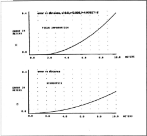
The second issue is whether the available accuracy at estimating 17 translates into a reasonabie accuracy in estimating depth. Figure 2 (a) show the theoretical error curve for the human eye, assuming the accuracy at estimating q reported in [4J . It can be seen that reasonable accuracy is available out to several meters. This curve should be compared to the accuracy curve for stereopsis, shown in Figure 2 (b ), again assuming human parameters. lt can be seen that the accuracies are comparable.

E. Human Pereeptlon

We have recently reported evidence demonstrating that people make use of the depth information contained in focal gradients [9] ; interestingly, the ecological salience of this optical gradient does not appear to have been previously reported in the scienti6c literature. The hypothesis that the human visual system makes signi6cant use of this cue to depth has been investigated in two experiments.

In the first experiment, pictures of naturalistic scenes were presented with various magnitude of focal gradient information. It was found that increasing the magnitude of the focal gradient results in increasing subjective depth . In the second experiment, subjects were shown a rightward rotating wireframe (Nekker) cube displayed in perspective on a CRT. Such a display may be perceived as either as a rigid object rotating to the right, or (surprisingly) as wobbling, non­ rigid object rotating to the Jett . Normally subjects see the rigid inter­ pretations most of the time, but when we introduced a focal gradient that favored the non-rigid interpretations, the non-rigid interpretations was seen almost as often as the rigid one.

An experiment demonstrating the importance of depth of field in human perception can be easily performed by tbe reader. First make a pinhole camera by poking a small, clean hole through a piece of still paper or meta!. Imposition of a pinhole in the line of sight causes the depth of lield to be very )arge, thus ellectively removing this depth cue from the image. Glose one eye and view the world through the pinhole, holding it as close as possible to the surface of your eye, and note your impression of depth (for those of you with glasses, things will Iook sharper if you are doing it correctly ). Now quickly remove the pinhole and view the world normally (still using only one eye). The cbange in the sense of depth is remarkable; many observers report that ·tbe change is nearly comparable to the difference between monocular and binocular viewing, or the change which occurs when a stationary object begins to move.

III. IMPLEMENTATION AND EVALUATION

A. Uslng sharp edges

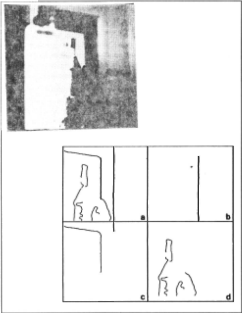
The first method of deriving depth from the focal gradient, by measuring apparent blur near sharp discontinuities, was implemented in a straighttorward manner (convolution values near zero-crossings were employed in Equations (4)- (6)) and evaluated on the image shown in Figure 3. ln this image the optical system bad a smaller depth of field than is currently typical in vision research; this was done because the algorithm requires that the digitization adequately resolve the point spread function .

Figure 3 also shows the depth estimates which were obtained when the algorithm was applied totbis image. Part (a) of this Figure 3 shows all the sharp discontinuities identilied [2] . lt was found tbat there was considerable variability in the depth estimates obtained along these contours, perhaps resulting from the substantial noise (3 of 8 bits) which was present in tbe digitized image values. To minimize this variability the zero-crossing contours were segmented at points of high curvature, and the depth values were averaged within the zero-crossing segments. Figure· 3 (b), (c), and (d) show the zero-crossing segments that have )arge, medium, and small deptb values, respectively . It can be seen that the image is properly segmented with respect to depth, with the exception of one small segment near the top of (c). This example demonstrates that this depth estimation technique - which requires Jittle computation beyond the calculation of zero-crossings - can be employed to order sharp edges by their depth values.

B. Comparlson of different apertures

The second technique, comparing two images identical except for aperture, can be implemented in many different ways. We will report a very simple version of the algorithm that is amenable to an inexpensive real-time implementation.

In this algorithm two images are acquired as shown in Figure 1 (a); they are identical except for their depth of field and thus the amount of focal gradient present, as shown in Figures 1 (b) and (c). Theseimages are thcn convolved with a small Laplacian filter, providing an estimate of their local high-frequency content. The output of the Laplacian filters are then summed over a small area and normalized by dividing them by the mean local image brightness, obtained by convolving the original images with a Gaussian filter. lt appears that a regionassmall as 4 x 4 pixels is sufficient to obtain stable estimates of high-frequency content. Figures 4 (a) and (b) show the normalized high-frequency content of Figures I (b) and (c).

Finally, the estimated high-frequency content of the blurry , large­ aperture image is divided by that of the sharp, small-aperture image, i.e., each point of Figure 4 (a) is divided by the corresponding point in Figure 4(b). This produces a "focal disparity" map, analogous to a stereo disparity map, that measures the change in focus between the two imagcs and whose values are monotonically related to depth by Equation (1). Figure 4 (c) shows the disparity map produced from Figures 2 (b) and 2 (c); intensity in this figureisproportional to depth.

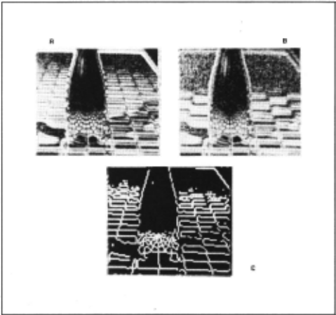
Areas of 4 (c) that are black have insufficient high-frequency energy in the sharp-focus image to make an estimate of depth.

lt can be seen that this disparity map is fairly accurate. Note that points reftected in the bottle are estimated as further than points along the edge of the bottle; this is not a mistake, for these points the distance traveled by the light is further than for those along the edge of the bottle. This algorithm, in common with stereo and motion algorithms, does not "know" about mirrored surfaces.

C. Design for a real-time lmplementatlon

A minimum of one convolution per image is required for this tech­ nique, together with a left shift and Cour subtractions for the Laplacian , and three divides for the normalization and comparison. Ir special con­ volution hardware is available, one can use two convolutions - one Laplacian and one Gaussian - per image, leaving only three divides· Cor the normalization and comparison. Frame buffers tbat can convolve image data in parallel with image acquisition are now available at a reasonable price, leaving as few as 3 operations per pixel to calculate the disparity map. For a 256 x 256 image, this can be accomplished in as little as 0.35 seconds with currently available microcomputers.

IV. DISCUSSION

The most striking aspect of this source of depth information is that absolute range can be estimated from a single view with no image-to­ image matehing problem, perhaps the major source of error in stereo and motion algorithms. Furthermore, no special scene characteristics need be assumed, so that the techniques utilizing this cue to depth can be generally applicable. The second most striking fact is the simplicity of these algorithms: it appears that a real-time implementation can be accomplished relatively cheaply.

Measurement of the focal gradients associated with limited depth of field appears to be capable of producing depth estimates that are at least roughly comparable to edge- or feature-based stereo and motion algoritbms. Tbe matbematics of tbe aperture-comparison tecbnique sbows it to be potentially more reliable tban stereo or motion - i.e., there is no correspondence problem, and one can obtain an interoal check on tbe answer - altbougb (as discussed above) it bas somewbat less accuracy.

· which can be done by table lookup.

The sharp-edge algoritbm appears to bave potential for useful depth-plane segmentation, altbougb it is probably not accurate enougb to produce a deptb map. I believe tbat tbis algoritbm will be of some interest because most of tbe work - 6nding and measuring tbe slope of zero-crossings - is often already being done for otber purposes. Tbus tbis type of depth-plane segmentation can be done almost as a side effect of edge 6nding or other Operations.

Tbe aperture-comparison algoritbm provides considerably stronger information about the scene because it overconstrains scene deptb, allowing an internal check on tbe algorithm's answer. Thus it provides depth information with a reliability comparable to the best that is theoretically available from tbree-or-more image stereo and motion algorithms, although it has ~".." "what less depth resolution. Tbe major Iimitation in measuring focal gradient deptb information in this manner appears to be insuring sufficient high-frequency information to measure the change between images; this requires having both adequate image resolution and bigh-frequency scene content.

Summary. In summary, we bave described a new source of depth information - tbe focal gradient - that can provide depth informa­ tion at least roughly comparable to stereo disparity or motion paral­ lax, while avoiding the image-to-image matehing problems that bave made stereo and motion algorithms uoreliable. We have shown that the limited depth of 6eld inherent in most optical systems can be used to make depth maps of useful accuracy with relatively minimal com­ putation, and have succesdully demonstrated a potentially real-time tecbnique for recovering depth maps from realistic imagery. It is our bope, therefore, that this research will prove to be a substantial ad­ vance towards building a robot that can function in complex, moving natural environments.