
Learning Intermediate Concepts in Constructing a Hierarchical Knowledge Base
Proceedings of the Ninth International Joint Conference on Artificial Intelligence. Learning and Acquisition. Pages 659-665.
© 1985 International Joint Conferences on Artificial Intelligence
Abstract
In expert systems. hierarchical reasoning can provide better accuracy a nd understandability. Here, we develop a method of learning hierarchical knowledge from a case library, in which each tr ain ing instance is described by low level features and high level concepts (e.g., manifestations and diseases) but not by intennediate concep ts (e.g., disease states). · Learning intennediate knowledge involves exploiting the o ld partial intennediate knowledge or creating new intennediate concepts by observing the relationship between the low level features and high level concepts. Experiments in the domain of diagnosing causes of jaundice validate the method.
- Clancey, W. 1. The epistemology of a rule-based expert system: A framework for explanation. Artificial Intelligence 20. 1983.
- Fu, Li-Min. Learning Object-level and Meta-level Knowledge in Expert Systems.
- Langley, P., Bradshaw, G. L., and Simon, H. A. Rediscovering chemistry with the BACON system. In Machine learning, chapter 10, . Tioga Publishing Company, Palo Alto, CA. 1983.
- Lenat, D. B. Theory formation by heuristic search. The nature of heuristics II: Background and examples. Artificial Intelligence 21, 1983.
- Michalski, R. S. Theory and Methodology of Inductive I .earning. In Machine Learning, chapter 4, . Tioga, Palo Alto. CA, 1983.
- Michalski 83b) Michalski. R. S. and Stepp, R. E. [Mitchell 78] [Utgoff82)
- Winston 70) Learning from observations: Conceptual clustering. In Machine learning, chapter 11. . Tioga Publishing Company, Palo Alto. CA. 1983.
- Mitchell. T. M. Version Spaces: An approach to concept/earning.
- Utgoff, P. E. Acquisition of appropriate bias for inductive concept learning. Technical Report, Thesis proposal, Department of Computer Science, Rutgers University. 1982.
- Winston, P. H. Learning structural descriptions/rom examples. Technical Report TR-76, Project MAC, MIT. 1970.
References were extracted automatically from the PDF and may contain errors.
Full text extracted automatically from the PDF; figures, tables and equations may differ. The PDF is the version of record.
LEARNING INTERMEDIATE CONCEPTS IN CONSTRUCTING A HIERARCHICAL KNOWLEDGE BASE
Li-M in Fu and Bruce G. Buchanan Computer Science Department Stanford University Stanford, CA 94305


HN: high level node (e.g .. diagnostic category) D IN: 1f intermediate level node IN : 1f LN : low level node (e.g., observational data)Abstract
In expert systems. hierarchical reasoning can provide better accuracy and understandability. Here, we develop a method of learning hierarchical knowledge from a case library, in which each training instance is described by low level features and high level concepts (e.g., manifestations and diseases) but not by intennediate concepts (e.g., disease states). · Learning intennediate knowledge involves exploiting the old partial intennediate knowledge or creating new intennediate concepts by observing the relationship between the low level features and high level concepts. Experiments in the domain of diagnosing causes of jaundice validate the method.
INTRODUCTION
In expert systems. hierarchical reasoning can provide better accuracy and understandability. Descriptions of intennediate states partially summarize and categorize subsets of the data and thus allow a reasoning system to reason from initial data to final conclusions in orderly stages. In MYCIN, for example, an inferred intennediate state of the patient is "compromised host" . i.e .. a person whose immune system has been lowered. It is neither a piece of primary, observed data (called here a low level node) nor a final diagnostic category (called here a high level node). Using intennediate nodes (IN's) allows the reasoning to proceed in smaller steps. It also allows the system to exploit the familiarity of some IN's for purposes of explanation [Clancey 83]. Finally, IN's may provide a partial interpretation of the data that is useful even when insufficient data are available for a complete interpretation. The reasoning hierarchy may be diagramed as figure l.
Intennediate nodes can be names of (a) generalized findings (e.g., clinical syndromes, which often start out as almost arbitrary labels for collections of findings): (b) generalized disease classes (e.g., MYCIN inferred "meningitis" before it inferred "bacterial meningitis"); (c) intennediate concepts that are neither final solutions nor primary data (e.g., ,;compromised host" in MYCIN).
·This repon describes work done in the Computer Science Depanment at Stanford Lniversity. It was supponed in pan by the Advanced Research Project Agency under the contract DARPA N00039-83·C·Ol36. National Institute Health under the grant '-'I H RR ·00785·11. and National Aeronautic Space Administration under the grant NAG·5·26l. We are grateful for the computer time on the SUMEX·AIM resource.
Figure l. Multi -1 eve 1 reasoning network. Note that there may be several intermediate levels.
In building a knowledge base for an expert system, it is useful to include IN's for the three reasons just cited. If the knowledge base is built through knowledge engineering, an expert can supply the appropriate IN's. If it is constructed automatically. however, the learning program must be able to supply the IN's if the cases from which it learns are described in terms of LN's and categorized in terms of HN's. Thus the problem we are addressing in this paper can be described as:
Given: A set of training instances (or a set of LN -> HN) . Find: Rules of the form LN => IN and IN => HNconsistent with the training instances .
In the above fonnulation, "-)" represents a specific link in a training instance; "= )" represents general inferential knowledge (a rule). That is, we intend to learn general intennediate knowledge from a set of very specific descriptions. (Note that "LN" can be conjunction of more than one feature.) Practically, this is an important issue and worthwhile to explore because. for instance, medical records are often described only by clinical manifestations and disease diagnoses (there is no or limited discussion of the involved intennediate mechanisms).
Two sets of learning methods are described below to cover two important cases:
- L Intermediate nodes already exist in the initial vocabulary;
- Intermediate nodes are not in the initial vocabulary.
In the first situation, the learning task involves exploiting the old partial (incomplete) intermediate knowledge to learn new intermediate knowledge; the partial knowledge may exist between LN and IN, or between IN and HN, or both. The task in the second situation is comparatively more abstract and constructive. because it involves creating and defining new intermediate concepts which are not provided in the original vocabulary. In inductive concept learning. automatically adding new symbols is one way to mitigate the bias induced by the fixed language [Utgoff 82].
The link from manifestations to a disease (IN = > HN) is called an inference (or diagnostic) rule. the opposite (H N = > IN) is called a descriptive rule. We focus here on learning diagnostic rules that include intermediate concepts (i.e .. LN => IN => HN). We first describe the learning techniques when the intermediate concepts are already in the initial language, and then describe the method when the intermediate concepts are not in the language. Finally, we describe results in which learned rules are tested in the context of a program named JAUNDICE. an expert system for diagnosing the causes of jaundice (see [Fu 85)).
II INTERMEDIATE CONCEPTS IN THE INITIAL VOCABULARY
In this section. we assume there is some knowledge about the intermediate nodes (IN) including partial but not complete knowledge about their relationship with other nodes at other levels (LN or HN). We also assume each training instance is characterized only by LN and HN and not by IN. If each training instance is characterized with low level descriptions (LN) and the associated intermediate (IN) and high level concepts (HN). we can apply machine learning algorithms level by level and discover new knowledge in different levels.
Basically, two methods are used to search the space of connections of LN's to IN's and IN's to HN's: bottom-up and top-down. The bottom-up method relies on the existing knowledge of "LN < = > IN"; the top-down method relies on the existing knowledge of "IN < = > HN". Therefore, if only knowledge of linkages between LN's and IN's is available, only the bottom-up method can be used; likewise if only knowledge of linkages between IN's and HN's is available, only the top-down method can be used. If both types of knowledge are available (but incomplete, otherwise there is nothing to be learned). both methods can be applied and the results will be the union of results from each method. A third method called "bidirectional extension" employs these two basic methods bidirectionally and sequentially in order to construct more complex hierarchical concepts.
A. Bottom-Up Learning
If the knowledge about "LN => IN" is available. this method can be adopted. The task of learning under this situation is described as follows:
Given: 1. A set of training instances
(or a set of LN -> HN);
- Rules linking LN and IN, in the direction of LN => IN.
Find: Rules of the form IN => HN, consistent with the training instances.
Each training instance is represented as a set of LN's and is classified on the basis of some HN. Remember that HN is a class name (or a disease in medicine). The basic idea behind this method is to generalize from instances of the same HN. In the JAUNDICE experiments, a set of rules in the form of "LN = > HN" are tirst learned (the method is not described here for reasons of space; it is described in [Fu 85]) from the given set of training instances: then we treat this set of rules as another set of training instances (more general than the original training set. of course) and apply the following procedure to learn intermediate rules.
Suppose there are n HN's: HI. H2, ...... Hi . ...... Hn, in the set of final hypotheses. The algorithm proceeds as follows:
Fori=! ton. Do:
- ~ Label all instances associated with the class of Hi as positive instances and label other instances as negative instances.
- ~ Generalize from positive instances by using the concept hierarchical tree. The generalization should:
- o be maximally specific to avoid over-generalization:
- o be tested against negative instances.
Intermediate nodes are involved and intermediate links (IN = > HN) are discovered during the process of generalization via hierarchy (sec the following example).
Step 2 proceeds as follows:
- substep 2.1 Initialize the hypothesis space H with the set of all positive instances; i.e., each positive instance represents one hypothesis in H. For example, if hl is the first instance of class Hi, we formulate one hypothesis in H as follows: hl = > Hi. Each hypothesis in H is associated with a degree of certainty, which is estimated from the statistics among instances.
- substep 2.2 For each hypothesis hi in H (starting from the head of H), do the following:
- o Form set H· by finding all hypotheses in H with the same range of degree of certainty (±.15) as hi (H· excludes hi).
o For each element hj in H*, find the common maximally specific generalization (called hk) of hi and hj. hk is plausible if it does not break the following constraints: its associated degree of certainty is at least ".4" and in the same range as hi's and it should not cover more than 10% of all negative instances.·· If it is plausible, then retain it (hk), put it in the end ofH, and prune hi from H. If no element in H* can form a plausible generalization (without breaking the constraints above) with hi or H* is an empty set, then output hi as a new rule and prune it from H.
- substep 2.3 Also, remove redundant hypotheses from H.
- substep 2.4 Repeat substeps 2.2 and 2.3 until H is empty.
This data-driven algorithm differs from the version space approach [Mitchell 78) in that this algorithm considers not only that there may be multiple rules for each concept but also that an instance may be covered by several rules instead of a single rule.
In the following simplified example, we assume that no uncertainty is involved and that two hypotheses are mutually exclusive. (Both assumptions can be removed.)
Example l. Suppose there are three instances
in the instance space as follows: Xl: L1 -> Hl X2: L2 -> Hl
X3: L3 -> H2
A simple hierarchy is given by five rules, given two IN's (M and N) in the vocabulary and shown schematically as follows:
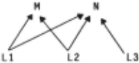
The following are two possible generalizations from Xl and X2:
Gl:M=>Hl
G2: N => Hl
G2 is not justified because if it is true, then L3 => N => Hl, contradicting X3.
Thus, the found link is: Gl: M => Hl.
·· We do not consider the minimal generality here because. as stated earlier. this method is applied to the set of rules learned; therefore they are already sufficiently general.
In JAUNDICE, for example, the two instances. "esophageal varices = > hepatic cirrhosis" and "ascites = > hepatic cirrhosis", may be generalized into "portal hypertension = > hepatic cirrhosis" by using the existing knowledge, "esophageal varices = > portal hypertension" and "ascites=> portal hypertension".
This technique is extended from the technique of climbing the generalization tree, which is used in other work, such as [Winston 70) and [Michalski 83a). However, we emphasize a concept hierarchy instead of a value hierarchy. Moreover, uncertainty may be involved in the hierarchy.
B. Top-Down Learning
If knowledge exists linking IN's and HN's, the technique of top down learning can be applied. The task is formulated as follows:
Given: 1. A set of training instances. (or a set of LN -> HN}; 2. Rules linking IN and HN, in the direction of HN => IN.
Find: Rules of the form LN => IN, consistent with the training instances.
In order to learn rules of the form of "LN = > IN", we may first. based on the available knowledge of "HN = > IN", re-label training instances such that they have new class names which are IN instead of HN. The algorithm used in learning "LN = > HN" is then applied to the transformed instances, and the results will be "LN =>IN" which is consistent with the training instances.
In JAUNDICE, for example, three diseases "acute hepatitis", "chronic hepatitis", and "hepatic cirrhosis", can be transformed into a common intermediate pathological category, "hepatocellular injury". and the inference rules for "hepatocellular injury" are learned from the same case library by the same learning method we use to learn the inference rules for each disease.
C. Bidirectional Extension Strategy
This strategy combines the bottom-up and top-down methods to learn more complex hierarchical concepts. Consider a four-level hierarchy as follows:
Suppose we have the knowledge of"LN <=> INievell" and "1Nievel2 < = > HN" (see figure 2) and each training instance is described by "LN -> HN".
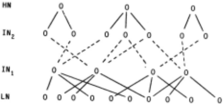
We can first learn "IN Ievell = > HN" by bottom-up method which exploits the existing knowledge of "LN < = > IN Ievell ... Then we treat all links of" IN Ievell = > HN" as another set of training instances, and we can learn the knowledge of" IN Ievell = > IN 1 evel 2 " by top-down method which exploits the existing knowledge of"IN 1 evel 2 <= > HN". Thus. we obtain all inferential knowledge "LN = > IN Ievell = > IN 1 evel 2 = > HN" from a set of training instances by extending the knowledge of only "LN <=> INievell" and "IN!evel2 <=> HN". If we view this learning task as a search, it actually proceeds bidirectionally. Whether the procedure starts bottom-up or top-down does not matter if we assume the training instances are correct and complete. In a domain without uncertainty, consider when inconsistency occurs in the following three instances (Hl and H2 are mutually exclusive): (Ll & Hl), (Ll & H2). and (L2 & Hl), and assume we have existing knowledge as follows: Ll = > I l, L2 = > I l, HI = > Ill, and H2 = > 112: then starting with the top-down method, we can first find the following consistent (i.e., no inconsistency) intermediate knowledge: L2 = > Ill, whereas starting with the bottom-up method, we find no consistent intermediate knowledge. In the current implementation, we ignore such inconsistency.
In the example of a four-level hierarchy, we can still obtain the knowledge of all levels by using the bottom-up method alone if only the knowledge of"LN <=> IN!evell" and "IN!evell <=> IN!evel2" is available, or by using the top-down method alone if only the knowledge of "1Nievel 2 <=> HN" and "IN!evell <=> IN!evel2" is available. Hence, it is possible to obtain even more complex hierarchical concepts by applying these two methods sequentially, depending on the available knowledge.
One example cited from JAUNDICE is as follows. Initially, there are three rules in the form of"LN => HN" : "malaise=> hepatitis". "fatigue => hepatitis". and "poor appetite => hepatitis". These rules are generalized to the form of" IN Ievell = > HN" by using the bottom-up method: "constitutional symptoms =>hepatitis". This rule subsequently results in another rule in the form of "IN Ievell => IN 1 evel 2 " by using the top-down method: "constitutional symptoms = > hepatocellular injury".
III INTERMEDIATE CONCEPTS NOT IN THE INITIAL VOCABULARY
Sometimes intermediate concepts arc not already specified in the initial vocabulary, so it is necessary to create and define them. The key issue is when and how to create new intermediate concepts. Two techniques are introduced: the technique of naming taxonomy I2Qiru:! and naming switchover oojnts. ·
A. Technique of Naming Taxonomy Points
We assume there are n classes of objects or concepts in the instance space. The algorithm proceeds as follows:
- ~ Construct a taxonomy tree on the basis of a similarity or dissimilarity measurement. One way of measuring dissimilarity is based on the of "sum of (the absolute value) of the differences of weighted individual features" (though non-linear functions can also be tried). First. based on the domain knowledge, select some important features and assign them weighting factors. Second, calculate the difference between the average value of an individual feature for the given two classes. If the feature values are not numerical. transform them into numerical values on the basis of domain knowledge. In medicine, this is a feasible approach because the clinical feature values can be quantized according to the clinical severity. (However, in some domains. symbolic measurements may be necessary. One example of clustering by a non-numerical technique is seen in [Michalski 83b].) For example. in JAUNDICE. the elevation of the serum enzyme is quantized into 0. L 2 and 3, representing normal, mildly-elevated. moderately elevated and highly-elevated. Third, calculate the sum of the differences of weighted individual features. Using different dissimilarity functions (i.e.. using different features or different weighting factors) may yield different results. So. it is possible to build more than one taxonomy tree.
Example 2. Computation of dissimilarity between two diseases in a library of four cases. The weights of the two features used are assumed equal here for simplicity.
Instance1: {(GOT 2) (Alk-P 0)} -> Disease A
Instance2: {(GOT 3) (Alk-P 1)} -> Disease A
Instance3: {(GOT 1) (Alk-P 2)}
-> Disease
8
Instance4: {(GOT 2) (Alk-P 2)} -> Disease 8
(where 0: normal
1: mildly abnormal
2: moderately abnormal
3: severely abnormal)
Compute as follows:
Average value for GOT :
Disease A: 2+3/2=2.5
Disease 8: 1+2/2=1.5
Average value for Alk-P:
Disease A: 0+1/2=.5
Disease 8: 2+2/2=2
Dissimilarity(A & 8}=(2.5-1.5) + (2- . 5) =2.5
Then we set up a criterion to group different classes in a common category if their mutual dissimilarities are smaller than a certain threshold. The criterion should be set in a way such that one class will not be grouped in two different categories. In a taxonomy tree. the tip nodes are HN in our terminology, and each non-tip node (excluding the root node) represents an IN.
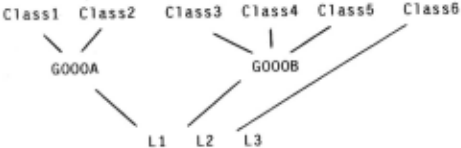
- step 2. Assign a symbol to every intermediate node in taxonomy tree, and thus create new intermediate concepts (IN) (see figure 3).
""' /
Figure3. Suppose a simple taxonomy tree is built for objects, the intermediate taxonomy points are named as GOOOA and GOOOB.
- ~The taxonomy tree gives us the knowledge about "HN => IN". For example, in figure 3, "if X is a member of class l then X is in category GOOOA". Therefore, we can apply the top-down method (described previously) and learn the knowledge of the form "LN => IN".
- ~Learn knowledge of the form "IN => HN" which is the link from IN (or mixed IN and LN) to HN by the following procedures:
- o First, Learn discrimination rules for different classes (HN) under the same intermediate category (i.e., under a higher taxonomical category) after removing all instances which do not belong to it. Thus, these rules are "local" rules in the sense that they are only good for a certain intermediate category. For example, in figure 3. we may learn classification rules for class l and class 2 in the category GOOOA by removing all instances that are not in the category GOOOA. Suppose we obtain such a classification rule for class 1 as follows:
- "If an object has attribute Ll then it belongs to class 1."
o Second, we actually can write a more specific rule as follows:
"If an object is in category GOOOA and has attribute Ll then it belongs to class 1 . "The algorithm may be applied level by level, and the results will become hierarchical: i.e., LN => IN!evell => IN!evell => .... => HN.
In JAUNDICE, by applying this technique to 72 cases, we found five concepts (see table l). Four symbols, after medical interpretation, were found to correspond to "hepatocellular injury", "cholestasis", "intrahepatic jaundice", and "extrahepatic jaundice" in the initial vocabulary of JAUNDICE. A fifth term, "hemo-gilb", was found because two diseases, "hemolysis" and "congenital conjugation defect (e.g., Gilbert's disease)" are similar and under the same taxonomy point. Though clinically meaningful (negative bilirubinuria), the symbol "hemo-gilb" bears little pathophysiological meaning.
| Symbols | Medical Interpretation· |
| Neosyml | Hepatocellular injury |
| Neosym2 | Cholestasis |
| Neosym3 | Intrahepatic jaundice |
| Neosym4 | Extrahepatic jaundice |
| Neosym5 | ? Hemo-gilb |
- ·· The interpretation depends on the diseases included by the symbol.
Note that this technique is intended to discover new intermediate concepts, but the concepts may have already been in the vocabulary. Hence, after new symbols are created, they should be checked whether they are equivalent to the old symbols semantically. Of course, this depends on the size of the case library, so we may want to keep redundant concepts around for a while.
B. Technique of Naming Switchover Points
The development of this technique is motivated by the observation that intermediate concepts often serve as switchover points between subsets of nodes in a reasoning network. One heuristic rule behind this technique is:
HRl: If i) There are subsets ofn LN's and m HN's such that all n LN's have (confirming) links to iill m HN's, ii) n>l and m>l and mn>4.
then it is worthwhile to define a common intermediate node.
Note that this is a cautious strategy in that every member of one subset is linked to every member of the other. We have not explored weaker forms of this heuristic that would increase the risk of incorrect inferences. This heuristic rule is also represented in figure 4.
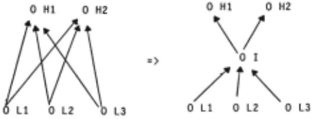
Since if one set of LN's (call it set L) and one set of HN's (call it set H) satisfy this rule, then any subset of set L and any subset of set H can also satisfy this rule, we detennine that the intennediate node be defined on the basis of the largest sets (subsets or supersets of set L and set H) of LN's and HN's which satisfy this rule. The second condition of this heuristic rule is, in fact. the threshold of the complexity of the relationship between LN and HN for defining new symbols. We deliberately choose this threshold because of the fact that, for a given situation which satisfies this rule, descriptions of the inference behavior are simplified by adding a common intennediate node while all links from LN's to HN's are maintained via the intennediate node (i.e .. no links from LN to HN are added or removed). For example, in figure 4, there are 6 links (LN = > HN) initially and 5 links (LN = > IN and IN = > HN) after introducing an intennediate node. Consider a case where there are 10 LN's and lO HN's and lOxlO= 100 links initially; only 20 links are needed after introducing a common intennediate node. But if n = 1 or m = 1 or nm = 4 (e.g., n = 2 and m = 2), the descriptions of inference behavior will not be simplified by adding a common intennediate node. Note that we can control the number of newly defined intennediate nodes (concepts) by adjusting the threshold of complexity for defining them (i.e., adjusting the second condition of the described heuristic rule).
Creating a new intennediate node will face another problem if uncertainty is involved. For the example shown in figure 4, the final degree of certainty of Hl and H2 concluded from Ll. L2 and L3 should remain approximately the same before and after introduction of intennediate concepts. The degrees of certainty (or CF) are assigned to new links in such a way as to preserve these final degrees of certainty. See [Fu 85) for details.
In our experiment, heuristic rule HRl is applied to a set of rules (LN => HN) which are learned from training instances (LN ·> HN), and can be applied recursively, as long as there are plausible switchover points, to fonn a multi·level network. By applying this technique to the jaundice domain, totally there are nine symbols created, which are shown in table 2. Medical tenninology has been introduced by the user. This renaming and using extstmg tenninology must be done carefully to avoid the confusion that usually arises when old tenns are used in new ways.
Among these nine created symbols, four symbols are outside the initial (old) vocabulary and five symbols are semantically equivalent to some old symbols. It is also noticed that there is some overlap of the results from the technique of naming taxonomy points and from the technique of naming switchover points. The fact that most of the created symbols are medically meaningful is expected because an
| Symbols | Medical Interpretation• |
| Neosyml | Benign hepatic pathology• |
| Neosym2 | Cholestasis |
| Neosym3 | Chronic liver failure |
| Neosym4 | Complete biliary obstruction• |
| Neosym5 | Extrahepatic jaundice |
| Neosym6 | Hepatobiliary pathology |
| Neosym7 | Liver cachexia• |
| Neosym8 | Inflammation• |
| Neosym9 | Hepatocellular injury |
- ·· The interpretation is made by observing the involved features (LN) and diseases (HN).
- : These symbols are outside the initial vocabulary.
intennediate symbol is created only when there is a regular relationship between LN and HN (represented by the heuristic rule): and most of these relationships have been discovered and named in the last 4000 years.
IV RESULTS
This section describes the application of the developed method to constructing a hierarchical knowledge base for a rule·based system named JAUNDICE, whose task is diagnosing causes of jaundice from clinical manifestations.
The procedures are as follows:
- step 1. Learn the direct inference rules (LN = > HN) from the given set of training instances (the method is described in [Fu 85)).
- step 2. Starting from partial or no intennediate knowledge, explore the intennediate knowledge by all methods that include bottom-up, top·down, bidirectional extension, naming taxonomy point. and naming switchover point, as much as possible. Two things are expected: first, some methods may not work because of incomplete knowledge, e.g., the bottom-up method cannot be adopted when knowledge of the fonn "LN = > IN" is missing; second, the results from different methods may be redundant. The first problem is handled simply by abandoning the methods that cannot apply. The second problem can be solved by checking and removing redundancy. The symbols created by naming taxonomy points and naming switchover points must be interpreted before checking redundancy with old symbols and new symbols already created. The interpretation can be made automatically by observing the involved LN and HN (see tables I and 2). At this stage, the knowledge base under construction has knowledge of three types: LN = > IN, IN=> HN. and LN = > HN.
- step 3. Replace direct rules (LN = > HN) by intermediate rules (LN = > IN, and IN = > HN) if they are equivalent. By "equivalent", we mean the same conclusion (HN) with the same strength (degree of certainty, allowing an error of"O.I5")can be reached, given a set of low-level features (LN). For instance, in JAUNDICE, a direct rule "negative bilirubinuria and elevated urobilinogen = > hemolysis" can be replaced by the rule "negative bilirubinuria and elevated urobilinogen = > overproduction of bilirubin" and the rule "overproduction of bilirubin =>hemolysis" . Note that one direct rule may be replaced by several intermediate rules.
After this procedure, the knowledge base contains hierarchical concepts, but will also contain some simple associations of the form "LN = > HN" which cannot be explained by intermediate concepts.
In the jaundice experiment, we constructed a hierarchical knowledge base from a training set of 72 jaundice cases collected from the medical literature. The automatically constructed knowledge base has 232 rules including 112 intermediate rules (rules involved with intermediate concepts). We then compared this new knowledge base with an old knowledge base of 141 rules, which was built by encoding medical knowledge from textbooks and journals and is also hierarchically structured. First. we tested each knowledge base on the original 72 cases; the diagnostic accuracy of the new vs. the old knowledge base is 97.2% vs. 84.7%. But since the new knowledge base is based on these 72 training cases, its better performance is somewhat expected. Therefore, we further tested the knowledge base on 68 other cases obtained from Stanford Medical Center; these cases received liver biopsy in 1978 and were not all diagnosable from clinical parameters alone. The diagnostic accuracy of the new vs. old knowledge base is 72.1% vs. 76.5%. Not every clinical case is clinically diagnosable because a disease may be in its incipient stage without full manifestation. Thus we remove all non diagnosable cases among these 68 cases, in which the pre-biopsy diagnosis made by the physician who sent the biopsy does not coincide with the biopsy diagnosis. (Although some error may be introduced by using the diagnosis of the attending physician as a "gold standard", this is preferable to the bias that would have been introduced if we had selected the cases that were not diagnosable from clinical parameters alone.) On the 42 remaining diagnosable cases, the diagnostic accuracy is 83.3% vs. 88.1 %. The result of "paired t test" shows "t= 1.434", which indicates the null hypothesis is accepted, or there is no significant difference between results obtained from the new KB and the old KB (see table 3). The 5% difference in results may be ascribed to the fact that many more cases than 72 are needed to learn rules for even a well-circumscribed domain. Textbooks. after all, encode summaries of considerably more experience.
| Old KB (141 rules-manually encoded from textbooks) | New KB (232 rules-automatically learned) | |
|---|---|---|
| Accuracy on training set for automatic learning (72 cases) | B4.7% | 97.2% |
| Accuracy on test set (68 cases) | 76 . 5% | 72.1% |
| Accuracy on test set with clinically diagnosable* cases only (42 cases) | 88.1% | 83 . 3% |
If we turn off the intermediate knowledge learner and learn only direct rules (i.e., only step 1 described above is turned on), we obtain a knowledge base of 185 (direct) rules; this knowledge base without intermediate knowledge can save execution time to some extent if compared with the knowledge base of 232 rules (recall that the average system execution time is roughly proportional to the number of rules in the knowledge base). Hut the diagnostic accuracy tested by the 42 diagnosable liver biopsy cases drops to 61.9% (vs. 83.3% if intermediate knowledge is added). Here, we may notice there is a tradeoff between execution time and quality of performance.
We further notice that cases which can be diagnosed correctly by the knowledge base with intermediate knowledge and cannot be diagnosed correctly without intermediate knowledge are cases with incomplete data. It seems clear that intermediate knowledge can improve the system prediction power particularly if only partial information is available. Moreover, intermediate knowledge provides much better understandability and explanation capability. For instance, in our experimental domain. the incorporation of intermediate knowledge can explain the underlying pathological and anatomical mechanisms of jaundice and make the diagnosis more convincing.
V RELATED WORK
Related work on creating new descriptors or concepts includes EURISKO [Lenat 83], BACON [Langley 83], and [Utgoff 82]. The principal difference is our explicit attempt to discover new intermediate concepts to construct a reasoning hierarchy. However, from the viewpoint of establishing a conceptual hierarchy, the most representative related work in AI is [Michalski 83b]. But it differs from our work in at least two aspects. First. our work deals with not only conceptual clustering but finding the intermediate links. Second, because each training instance is also characterized by a high level concept besides low level descriptions, the search for the meaningful intermediate concepts is constrained bidirectionally (from LN and from HN).
VI CONCLUSION
We expect the methods described here can be easily extended to non-medical domains. In learning intermediate knowledge, we use a general concept hierarchy; and the heuristics we use to discover intermediate knowledge are not specific to medicine. The major contribution of this idea is its capability of learning intermediate-level concepts from a set of training instances that are described only by low level features and high level concepts and not by any intermediate concept.
Acknowledgments
We thank Dr. Gabriel Garcia and Dr. Peter B. Gregory for providing us with liver biopsy cases in Stanford Medical Center, which were used to help validate the learning method presented here.
@inproceedings{ijcai1985p128,
  title     = {Learning Intermediate Concepts in Constructing a Hierarchical Knowledge Base},
  author    = {Fu, LiMin and Buchanan, Bruce G.},
  booktitle = {Proceedings of the Ninth International Joint Conference on
               Artificial Intelligence, {IJCAI-85}},
  publisher = {International Joint Conferences on Artificial Intelligence},
  editor    = {Aravind Joshi},
  pages     = {659--665},
  year      = {1985},
  note      = {Learning and Acquisition},
  url       = {https://ijcai.org/proceedings/1985/128},
}
TY - CPAPER TI - Learning Intermediate Concepts in Constructing a Hierarchical Knowledge Base AU - Fu, LiMin AU - Buchanan, Bruce G. T2 - Proceedings of the Ninth International Joint Conference on Artificial Intelligence, IJCAI-85 PB - International Joint Conferences on Artificial Intelligence PY - 1985 SP - 659 EP - 665 UR - https://ijcai.org/proceedings/1985/128 ER -Copied
Machine-readable versions of this paper, for tools and AI agents:
 Welcome
 Future Conferences
 AI Journal Division
 IJCAI Proceedings
 About IJCAI
 IJCAI Awards