A Diagnosis Method of Dynamic System Using the Knowledge on System Description

1. Component Description

Each component is deisgnated by an atomic name and its type is specified by Type statement. Three examples are given below.

<Type A Sensor> <Type B Selector> <Type C Pump>

2. Connectivity Description

Each component has zero or more inputs and outputs. Connectivity relation­ ship among components is specified by Conn statement. One example' is given below.

(Conn <output 1 Cl (input 2 All

3. State Description

Some components need information about their states. This information refers to on/off state, observability, redundancy, swithcing condition, etc ·. Four examples are given below.

<Value (input 1 Al on>

<Observable <value (output 1 Blll

<Redundant C D)

(Switchable <value (input 1 B>>>

B. Behavior Description

The behavior of a system is specified by describing the relationship between its input<s> and output(s) of each component

in terms of rules. Behavior of a component in a dynamic system is usually described by a differential equation, which is often discretized to a set of arithmetic expressions.

1. Dynamics Description

The rules relating input<sl to output<sl are denoted as forward behavior rules <FB rules> and these relating output(sl to input(sl as backward behavior rules <BB rules). Simulation of the sys­ tem behavior requests use of the FB rules but inference requests use of both rules. Use of the BB rules is encountered in inferring unobervable input(sl to a com­ ponent from observable output(s) of sensor(s).

a. Forward Behavior Rules

Two examples are given. The first is a sensor behavior and the second a con­ troller behavior. OK means that a com­ ponent is not faulty. Symbols starting with $ mean that these are variables. The statement <True A Bl means that A is true in situation B.

The first rule says that the sensor is a two-input, one-output device, one input being an on/off switch and the other sensing a quantity mi, and that if the sensor is on and functioning normally, the output mo is mi/mr, where mr is a scale factor. This is true for every t. The second rule is more complicated. The out­ put of the controller mo at time t is com­ puted by a function f that req~ires 6 variables, one of which is the output mi itself at the previous time step s. In these rules meta-knowledge is used to determine where to perform numeric compu­

tation.

(if <Type $X Sensor) (if <and <OK $xl <Value (input 1 $x) on) <True <value (input 2 $xl $mi) $t) <Value <rated $x> $mrl <= $mo (/ $mi $mr>>> <True <value <output 1 $x) $mo) $t))) (if <Type $X Controller) (if (and <OK $X) <True <value (input 2 $X) $lll $sl <True <value (input 3 $X) $wfl) $s) <True <value <input 4 $X) $wml> $s) <True <value (output 1 $xl $ml) $s) <Value (input 1 $X) $ldl (= $t (+ $s 1)) <True <value (input 2 $x> $lo) $t) <= $mo f($ml $11 $lo $ld $wfl $wml) > > <True <value (output 1 $X) $mo> $t)))

b. Backward Behavior Rules

The following rule coresponds to the first example above.

(if <Type $x Sensor> ( if ( and ( OK $X) (True <value <output 1 $xl $mol $tl <Value (input 1 $x> on> <Value <rated $X) $rnr> <= $rni <*$rna $rnr>>>

<True <value (input 2 $xl $mil $t)))

2. Connectivity Description

· There needs a set of rules that interprets the connectivity relationship. These are rules that if two ports are con­ nected, they always bear the same value.

a. Forward Connectivity Rule <FC rule)

• (if <and <Conn $X $yl <True <value $x $zl $tll <True <value $y $zl $tll

b. Backward Connectivity Rule <BC rule)

• (if <and (Conn $x $y> <True <value $y $zl $tll

<True <value $X $zl $tll

IV METHOD OF DIAGNOSIS

The diagnosis consists of the following four steps. ·

A. Computation of Expectation Value

Start of diagnosis is an interpreta­ tion that the symptom does not match the expectation. It is, therefore, necessary to estimate the expected value of the sen­ sor where an anomaly is detected. To do this, plant dynamics has to be simulated starting from some initial state. It is not necessary to go back to a state where all components were normal because the input and output relationship of a normal component is consistent regardless of the value · of its input(s). It is sufficient, in a dynamic system having feedback loops, to go back at least to the time t-2~ and use a set of consistent observable data, where t is the time of anomaly detection and ~ is the maximum difference of time for input(s) of any component to affect output<s> of any other component including itself in solving the dynamics by time discretization.

Inference is made in two steps. First, forward chaining is applied to obtain unobservable data at time t-2~ starting from the observable da~a at time t-2~ using the structure data, BB and BC rules assuming all components are normal. Next, forward chaining is applied to obtain the expectation value of the ano­ maly detected sensor at time t starting from the estimated unobservable data using the structure data, FB and FC rules.

B. Computation of Suspects

Using the fact that the symptom is against the expectation, all components that can logically be responsible for the symptom are picked up as suspects. Linear input resolution is applied starting from the expectation violation at time t until it reaches the estimated unobservable data at time t-2~ using the structure data, FB and FC rules. All rules are converted to conjunctive normal form.

C. Discrimination of the Suspects Using Observable Data

It is possible to discriminate the suspects by checking the consistency of the available observable data. Here, con­ sistency means that the observed output<s> can be expected from the observed input(s) using the knowledge on system description. The knowledge required in this step is the structure data, FB, BB, FC and BC rules.

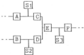
Inference is made in two steps. First, a set of observable data required to identify the anomaly of one or more components is searched. Symbolic ~imula­ tion is performed by resolution starting from the FB rule of any one of the suspect candidates. Because the feedback nature of the system necessitates con­ current use of both forward and backward rules, inference should be controlled to avoid to get into an infinite loop. In Fig. 1, for example, starting the resolu­ tion from the component C, the sensors Sl, S2 and 53 are picked up as the data that

Si

.. A - F .·

Sensors

Suspects

Fig. 1 An example of the suspect discriminatiori by observa­ ble data can be used to identify anomaly in the components C, D and E. The sensors them­ selves can also be suspects in this case. This process is repeated until all suspects are grouped into smaller sets. Next, numeric simulation is performed for each set again using resolution to sheck if the observable data are consistent to each other. If they are not consistent, at least one of the components for that set is faulty.

D. Discrimination of the Suspects by Gen­ erating Tests

It is possible to further discrim­ inate the suspects by placing single fault and non-intermittency assumptions for each set if a meaningful test can be generated and if it is successful. Use of the redun­ dant component or valve open/close can be a realizable test in a plant diagnosis.

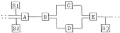
Inference is made in two steps. First, test form is generated. The knowledge required and the inference pro­ cedure used in this step are the same as in IV C. Figure 2 is an example of a set of suspects in which a test is possible.

Si Sensors

E Selector

Fig. 2 An example of the suspect discrimination by generat­ ing a test

The components C and D are redundant. Assume that the component C has been selected. The suspects at this stage are A, B, C and E. If there is still incon­ sistency among the data when the selector E is switched from C to D, the compponent C is exonerated from the suspects. Other­ wise, the component C is faulty. The resolution starts from the redundant com­ ponent D which is selected by the knowledge that C and D are redundant, the selector E is switchable and now C is selected, and is continued until the test form is obtained. Similar test can be gen­ erated in case of valve control. Next, numeric simulation is performed using resolution, and the simulated results is evaluated against the observable data.

V APPLICATION TO A DIAGNOSIS OF A NUCLEAR REACTOR POWER PLANT

The above method is applied to a sim­ plified model of feed-water system of a boiling water reactor shown in Fig. 3. Steam going out of the core is returned to the core by the feed-water pump after being condensed to water. Small fraction of the vapor is used to drive a turbine­ driven feed-water pump. The power level is controlled by recirculation flow rate. The water level is kept constant by the con­ troller which uses signals from water level sensor, feed-water flow meter and main steam flow meter. The condenser is assumed to serve as a source and a sink of water and vapor. The system dynamics are, thus, determined by those of the core, the controller and the pumps. The water level sensor 1 (53) and 2 (54), and the turbine-driven (J) and motor-driven <L> pumps are redundant components. In the normal operating condition, S3 and J are used. When S3 is used, 54 is not observ­ able.

The following hypothetical situation is assumed. The component S3 happened to fail. The anomaly was first detected by the alarm signal of S9 at the feed-water pump outlet during a load following opera­ tion in which the plant was not in a steady state. By the time of detection, the anomaly had already propagated through various components and affected many sen­ sor outputs although they were still within their allowable ranges except for S9.

After computing the expectation value of S9 using the past observable data (step 1), the suspects computation starts and returns the following components (step 2):

A, B, C, D, E, F, G, H, I, J, K, L, M, N, 0, Q, T, Sl, S2, S3, S8, S9

Use of the observable data discrim­ inates the suspects to the following seven (step 3):

A test is then generated knowing that S3 and S4 are redundant and S3 is in use:

[Switch the selector E to S4 from S3. If the data Sl, S2 and 54 are consistent, S3 is faulty. Otherwise, the fault must lie in one of A, B, C, D, Sl, S2 and S3.J

In this case, the data are consistent by the assumption, and thus, the test is successful. The faulty component is con­ cluded to be the water level sensor 1.

All of the above diagnosis steps are automated. To improve the efficiency, heuristic knowledge is also employed and used together with the knowledge on system description. An example is a knowledge that it is worth to start resolution from the redundant component in discriminating the suspects using the observable data.

VI CONCLUSION

A method to diagnose a dynamic system with feedback structure is proposed. The method neither require a fault model nor knowledge concerning failure causality. The diagnosis is mainly based on linear input resolution with explicit meta-level control and all of the inference steps are automated.

Application to a BWR feed-water sys­ tem demonstrates its diagnostic capability although the model is much simplified and the assumed anomaly is hypotheti­ cal.

Experience with example recommends combinatory use of heuristic knowledge for efficiency improvement. Employment of frame type representation of the system coupled with criteriality inference capa­ bilty would further improve the effi­ ciency. It is important to distinguish logical inference from simulation.

ACKNOWLEDGEMENTS

This paper is based on the work per­ formed at Teknowledge. Authors are grate­ ful for Profs. M. R. 'Genesereth and E. H. Shortliffe of Stanford University for their consultation. They extend their thanks to Drs. T. Kiguchi and S. Kobayashi for their critical discussions, and to Drs. S. Yamada and K. Taniguchi for their support of this work.