
Characterizing Search Spaces
Proceedings of the Eighth International Joint Conference on Artificial Intelligence. Planning and Search. Pages 780-781.
© 1983 International Joint Conferences on Artificial Intelligence
Abstract
A heuristic is good on a search space to the extent that it allows the prediction of which states are near to the goal. In this paper heuristics are investigated on several different search spaces. A measure is proposed for assessing the predictive accuracy of a given heuri stic on a given search space. Themeasure sheds light on characteristics of the Traveling Salesman Problem that make it computationally mor e difficult to solve than the Minimum Spanning-Tree Problem.
- Banerji, R B (1982) "Theory of Problem Solving: A Branch of Artificial Intelligence" Proc IEEE, 70: 12 p 1428-1448.
- Garey, M and Johnson, D (1979) Computers and Intractability Freeman & Co : San Francisco. Handbook of Artificial Intelligence, Vol/ (1981) ed A Barr and E Feigenbaum, William Kaufmann, Inc : Los Altos, Calif.
- Knuth, D E (1973) The Art of Computer Programming, Vol 3, Sorting and Searching, Addison-Wesley: Reading, Mass.
- Lenat, Douglas (1982) "The Nature of Heuristics " Artificial Intelligence, 19 189-249.
- Minsky, Marvin and Papert, Seymour (1972) Perceptrons , MIT Press: Massachusetts.
- Pearl, Judea (1983) "On the Discovery and Generation of Certain Heuristics" The AI Magazine, 4: I p 23-33.
- Nilsson, Nils (1980) Principles of Artificial Intelligence Tioga : Palo Alto, Calif.
- Rada, Roy (1981) "Searching and Gradualness " BioSystems, 14 p 219-226.
- Reingold, E, Nievergelt, J, and Deo, N (1977) Combinatorial Algorithms Prentice-Hall: Englewood Cliffs, New Jersey .
References were extracted automatically from the PDF and may contain errors.
Full text extracted automatically from the PDF; figures, tables and equations may differ. The PDF is the version of record.
CHARACTERIZING SEARCH SPACES
Roy Rada Department of Computer Science Wayne State University Detroit, Michigan 48202
ordering imposed by f on S ;, and to quantify this comparison, inversions are used. Let a 1, ··· , a" be a permutation of the set {1, . . . , n}. If i < j and a; > ai· then the pair (a ;,ai) is called an inversion of the permutation (Knuth, '73). For example, the permutation 2, 4, I, 3 has the three inversions (2, 1), (4,1), (4,3) .
To determine NIV k(S;J) the following 3 steps are performed:
i) Order all s t S; so thatf(s 1) :5 /(s2) :5 · · · /(sm) ·
ii) Compute h for each s and create the sequence h(s 1), h(s2) , ... , h(sm), where/(si) ::; /(su + n>· If /(si) = /(si + 1), then h(si) ::; h(si + 1).
iii) NIV k(S;J) = number of inversions in the sequence h(s 1), ... , h(sk).
Consider an ordering A = a 1, ··· , an and a permutation A ' = ~ 1 , ··· ,a; 11 · Define NIVi(A') to be the total number of inversions in a; 1 , ·· · , a;r In other words, NIV i(A') is the number of inversions in the first j elements of A'.
Theorem:
Given A' and NIV iA '), ... , NIV 11 (A'),
the list A can be constructed.
Proof:
Basis:
lfNIV 2 = l,thena; 1 ,a; 2 -+ a; 2 ,a; 1 , else ai 1 ,ai 2 _..., ai 1 , ai 2 ·
This makes the first two elements correctly ordered.
Inductive Step:
Assume the first k elements are correctly ordered.
Move a;<k + 11 to the left NIV (k + 11(A')-NIV k(A') positions.
Now the first k +I elements are correctly ordered.
Thus, one deals at each stage with just the total number of inversions--a scalar--and not the actual inversions which form a set of ordered pairs. Yet, from these scalars and A', A can be reconstructed.
RESULTS
ABSTRACT
A heuristic is good on a search space to the extent that it allows the prediction of which states are near to the goal. In this paper heuristics are investigated on several different search spaces. A measure is proposed for assessing the predictive accuracy of a given heuristic on a given search space. The measure sheds light on characteristics of the Traveling Salesman Problem that make it computationally more difficult to solve than the Minimum Spanning-Tree Problem.
INTRODUCTION
A search space SS is a quadruple (S, 0, I, G), where S is a set of states, 0 is a set of operators for moving from state to state, I is a set of initial states, and G is a set of goal states (see Handbook AI, '81 and Banerji, '82). The problem is to find the sequence of operators that connects some initial state to a goal state. To avoid exhaustive search, the search algorithm employs, as a guide, a heuristic evaluation function f (Nilsson, '80) .
To characterize the utility of f on SS a measure NIV is created. The author hypothesizes that difficult problems can be distinguished from easy problems with NIV. Difficulty is traditionally related to computational complexity, but NIV directly characterizes relationships within the search space.
FORMALIZATION
NIV on (SS, f) tells the degree to which similar states have similar /values . Two states are similar, if they are connected by an operator. To handle "similar" for f values the following terms are introduced: equivalence classes of states, heuristi~-predictions, and inversions. The equivalence class S ; is defined to be { s I s t S and s can be reached from I by a sequence of i operations } The heuristic-prediction function h on s t Sis h(s) = max { f(w) I w t S i+ 1 and I move connects s to w } . The ordering imposed by h on S; is compared to the
This work was supported in part by a Wayne State University Faculty Development Grant.
MSTand TS
Two important graph problems are the Minimum-cost Spanning Tree Problem (MST) and the Traveling Salesman Problem {TS). Both involve weighted graphs and the search for a subgraph with certain properties. In the MST a subgraph is desired that spans the graph and has minimal cost. In the TS a cycle is desired that crosses every vertex and has minimal cost. For a graph with e edges, the solution to the MST requires O(eloge) time steps. The only known algorithms to solve the TS require more than a polynomial amount of time (Garey and Johnson, '79) Why are these two problems of such different time complexity?
For many combinatorial problems Sis part of a power set P on some primitives. Consider, for example, the complete 4-node graph with edges a, b, ... , f and weights w(a), .. . , w(f). S MST = {sIs f P({(a,w(a)), ... , (f,w(f))}) and ls i ::; 3 }. In order that SMsT = STs· a modified TS is henceforth considered in this paper, where the goal on an n-node graph has n-1 edges. This modified TS is also NP-complete (Garey and Johnson, '79). A reasonable/forTS follows:
fTs({(xl>w(x1)), ... , (x i,w(xi))})
- = (w(x 1) + · · · w(xj))·1, if xi> . . . , xi contains no cycles or trisections
- = 0, otherwise.
| su | si.J | 51.7 |
| 3·1 | 4·1 | 8·1 |
| IJ ·I | IJ ·I | IJ ·I |
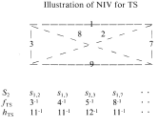
The reader is welcome to verify that for the weighted-graph of Figure I NJV iS2,/TS) = 0 and NIV 4(S2,/Ts) = I.
A computer program was written to determine NIV on MST and TS. The program generated complete graphs over 5 nodes. Weights were assigned to the edges after having been randomly chosen from a uniform distribution over {1, 2, .. . , 1000}. Eighteen graphs selected in this way had an average NIVi(S2,/Ts) > NIVi(S2,/MsT) for all j in S2 (see figure 2).
NJV versus Position
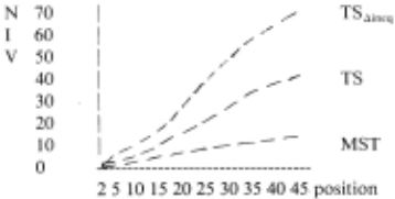
For S3 the relationship between NIV i(S3JTs) and N!Vi(S3JMsT) is similar to that for S 2. This evidence supports the hypothesis that more difficult problems have more NJV. However, at any given position j there exists a graph such that NJV i(SJTs) < N!Vi(S,J MST ), where i f { 2,3}. Just the average over the 18 graphs is consistently, significantly higher forTS than for MST.
Graphs were also studied whose edge weights satisfy the triangle inequality (t. ineq) . Approximation algorithms for TS aineq can propose a solution whose length is guaranteed to not be greater than 1.5 times the length of an optimal tour (Reingold, et al, '77). No such algorithms exist for the unconstrained TS. Thus one suspects that by some standard of Sllarch space "difficulty" D that D(MST) < D(TS aincq) < D(TS). This author hypothesized that NIV would order these 3 problems as D did. To investigate this hypothesis the computer program was amended to generate 18 graphs whose edge weights satisfied the t. ineq. For each graph the program chose 5 nodes whose coordinates were randomly chosen from the set {I, ... , 707}. The edge weights thus ranged from I to 1000.
The results did not support the hypothesis. The average NJV over the IS graphs revealed: N IV i(S2, TSt>incq) > N IV i(S2, TS), j f {3, ... ,45} (see Figure 2). The author does not know how to explain this data. Three possibilities are:
- The data showed NIV 2(S2, TSaincq) < NJV 2(S2, TS), which supports the hypothesis. The first two pos1ttons, as measured by NJV 2, have great bearing on problem difficulty.
- The weights in the TS aincq tests were not uniformly distributed over {I, .. . , 1000} but clustered into a smaller range . This may make the problem more difficult.
- TSaineq may be in important ways more difficult than TS.
Function Optimization
The perceptron learning algorithm can be viewed as a function optimizer. Minsky and Papert (' 72) showed that the search space of the perceptron is smooth and unimodal. The learning component of Samuel 's checker pl~yer is similar to a perceptron. A number of developments in the history of AI can be viewed as developments in function optimization. A simple example shows how SS, f, and NIV apply to optimization of discrete functions. Two functions were studied: one had I peak and the other had 4 peaks. One expects that the multimodal function is harder to optimize, and the author 's experiments produced a larger NJV for the multimodal function. S was the power set over all (x,y) pairs defining the function to be optimized. A set of initial (x,y) pairs formed /. 0 took a states , = {(xl>yl> ... , (x,,y;)} to {(x~>y 1 ), ... ,(x,,y;), (x;+1,Y; + 1)}, such that x, . 1 was "near" an x in s,. G was the (x,y) pair whose y was maximal. The heuristic wasf(s) = max{y I (x,y) f s}.
Rule-based Planning
Rule-based planning systems, like STRIPS and DCOMP (Nilsson, '80), fit the framework of this paper. For a simple example, denote the registers of a computer by r ; and the contents of r, by c,. The S of SS is {(r 1,c1), (r2,c2), (rl>cJ), (r.,c. )}, where c, f {0, a, b}. The initial state is {(r ~>a), (r2,b), (rJ,O), (r 4 ,0}}. One exchange problem E 1 has the goal of {(r 1,0), (r2,0), (r 3 ,a), (r 4 ,b)} . Another exchange problem E 2 has the goal of { (r 1 ,b), (r2,a), (r 3 ,0), (r4,0)}. The operator is the assignment rule in Nilsson (' 80):
| rule: | assign (r,,a,ri,b) |
| precondition: | (r,,a), (ri,b) |
| delete: | (r,,a) |
| assert: | (r,,b) |
The heuri stic f(s) tells the number of registers in s whose contents are the same as the corresponding registers in the goal. Both E 1 and E 2 can be solved in 4 steps. E 2 seems harder, since for it a step from S; to s; + 1 must be made such that h(s ;) > h(s; " 1 ). Application of NlV to E 1 and E2 reveals that NlY is much higher for E 2 than E1· This support s the hypothesis that NlY distinguishes problems by their difficulty .
Extensions: Backward-chaining and Search Algorithms
The definition of heuristic-prediction h involves looking from S; to S,+ 1 and thus is related to forward-chaining. A small amendment to h requires the new function bh to look backward from S; to 5; 1· ForsE S;, bh(s) = max{ f(w) I w E S ;.1 and sand w are connected by 0} . For all of the previously mentioned experiments, bh, as well ash, was used. When h is replaced by bh in the definition of NIV, a new function, called BNIV, is produced. For the function optimization and rule-based problems BNIY showed the same tendencies as NIY did--namely, the values of BNIV on the harder problems were larger than on the easier problems. BNIV for TS is not everywhere bigger than BNIY for MST. If step 2 in the definition of BNIV (and NIY) is amended so that f(s ;) = f(s; + 1) --> bh(s;) ?: bh(s;+ 1), then BNIY (and NIY) of TS is everywhere greater than BNIV (and NIV) of MST.
Another direction in which to extend the applicability of NIY is that of relating the performance of search algorithms to the NIY of search spaces. Consider a class of search algorithms A = {A1, A2, ·· · }. Each A; proceeds through an (SSJ) for which the state spaceS has been divided into equivalence classes S;, as defined earlier. Furthermore, A ; goes from S 1 to 5 2 to · · · Sk by emphasizing the states in each equivalence class whose f value places those states in the top i positions. One can show that over all possible SS and f those on which A ; performs well have, on the average, smaller NIY values than those on which A ; + 1 performs well. Details of this argument can be found in (Rada, '81 ).
DISCUSSION
An efficient search algorithm examines only a relatively small number of the states in a search space before finding a solution. Heuristics permit a search to explore efficiently, but a given heuristic is good for some problems and not for others. How can one characterize a heuristic's power vis-a-vis a particular class of search spaces? A heuristic must, in some sense, predict which states in the search space are close to the goals. Often, easily-solved problems are those for which a heuristic f exists such that similar states have similar f values (see the continuity argument of Lenat, '82) . This "similar-state --> similar-value" notion has been formalized in this paper by the introduction of predictions and a measure NIV, where NIY quantifies the accuracy of the predictions.
The hypothesis of this paper is that NIV can distinguish problems by their difficulty. Theoretical considerations reveal that for a search space and heuristic on which depth-first, best-first search finds the solution, NIV iS;. f) = 0, for all j. An easy problem, like MST, has the property that NIV 2(5;. f) = 0, for all j. To further test the validity of the hypothesis that NIV varies in proportion to problem difficulty, a large number of experiments have been performed . Three famous combinatorial graph problems, MST, TS ~;ncq· and TS, were analyzed on the computer. The computational complexity of MST is less than that of TS, and NIY for MST proves experimentally to be less, on the average, than NIV for TS. The experiments also demonstrate several phenomena which require more study before they can be considered evidence for or against the hypothesis. To demonstrate the applicability of this paper 's methodology on other than graph problems, function optimization and rule-based planning have been tested ; the results support the hypothesis .
Characterizing the utility of heurist ics is an important step in the development of a theory of heuristics. Constraints in a search space must be advantageously utilized by good search algorithms (Pearl, '83). By noting what a heuristic says about the search spaces on which it is useful (as NIY does), one may begin to understand how a heurist ic benefits from constraints. One next step towards a theory of heuristics and search spaces is to characterize hard and easy problems by their NIY values.
- Acknowledgements: Thanks to the referees and graduate student Ching-Chio Sheu.
@inproceedings{ijcai1983p189,
  title     = {Characterizing Search Spaces},
  author    = {Rada, Roy},
  booktitle = {Proceedings of the Eighth International Joint Conference on
               Artificial Intelligence, {IJCAI-83}},
  publisher = {International Joint Conferences on Artificial Intelligence},
  editor    = {Alan Bundy},
  pages     = {780--781},
  year      = {1983},
  note      = {Planning and Search},
  url       = {https://ijcai.org/proceedings/1983/189},
}
TY - CPAPER TI - Characterizing Search Spaces AU - Rada, Roy T2 - Proceedings of the Eighth International Joint Conference on Artificial Intelligence, IJCAI-83 PB - International Joint Conferences on Artificial Intelligence PY - 1983 SP - 780 EP - 781 UR - https://ijcai.org/proceedings/1983/189 ER -Copied
Machine-readable versions of this paper, for tools and AI agents:
 Welcome
 Future Conferences
 AI Journal Division
 IJCAI Proceedings
 About IJCAI
 IJCAI Awards