
A Knowledge Directed Line Finder for Analysis of Complex Scenes
Proceedings of the Sixth International Joint Conference on Artificial Intelligence. .
© 1979 International Joint Conferences on Artificial Intelligence
Abstract
As a part of complex scene analysis system, this paper presents a line finder which can find a globally good line with respect to the knowledge available of the line to be sought. A variety of knowledge available of the line to be sought can be communicated to the llne finding system simply in the form of descriptions so that the higher level of the program can easily use this line finding system. The optimization method is utilized to detect a globally good line with respect to the given knowledge of the line. In order to reduce the required storage space and computation time in the optimization process, we use the following techniques: I) represect a line by a sequence of linear segments and find the good sequence of segments by the optimization method and 2) use a locus model of search to prune unpromising lines during the optimization process. Some experimental results applied to various scenes with different amount of noise and knowledge are given in the paper.
- A. Martelli : An Appllcation of Heuristic Search Methods to Edge and Contour Detection, Commu. ACM 19, pp. 73-83, 1976.
- U . Montanari : On the Optimum Detection of Curves in Noisy Pictures, Commu. ACM 14, pp. 335-345, 1971.
- A. Martelli : Edge Detection Using Heuristic Search Methods, Comput. Grap. Image Proc. 1, pp. 169-182, 1972.
- S.M. Rubin and R. Reddy: The Locus Model of Search and Its Use in Image Interpretation, Proc. 5th IJCAI, pp. 590-595, 1977. IJCAI
- M. Yachida and S. Tsuji : A Versatile Machine Vision System for Complex Industrial Parts , IEEE Trans. C-26, pp. 881-894, 1977.
- M. D. Kelly : Edge Detection in Pictures by Computer Using Planning, in Machine Intelligence, 6, pp. 379-409, 1971.
- A. K. Griffith : Edge Detection in Simple Scenes Using a Priori Information, IEEE Trans. C-22, pp. 371-381, 1973.
- S. Tsuji and F . Matsumoto: Detection of Ellipses by a Modified Hough Transformation, IEEE Trans. C-27, pp. 777-781, 1978.
References were extracted automatically from the PDF and may contain errors.
Full text extracted automatically from the PDF; figures, tables and equations may differ. The PDF is the version of record.
1. llfTRODUCTION
Boundary detection is an important and critical stage in scene analysis to segment an input picture into meaningful regions. This process usually consists of the following two steps: (1) detection of short edge elements, and (2) connecting these edge elements into boundaries. Many methods have been proposed to detect short edge elements which apply local operations to every point of the input picture. An operator tuned up for characters of edges to be detected is usually used to enhance the edges to be sought in noisy pictures. In order to detect edge elements in noisy pictures, relatively large operators are often used to examine statistic properties of local regions. When edge elements have been found, then they are connected to form boundaries or lines. This line finding process must utilize properties about lines to be detected and must find globally good lines with regards to the properties in order to distinguish meaningful edges in noisy pictures. These properties of the lines to be sought must be separated from the line finding program and given in the form of data to the program, since minor changes of the characteristics of the sought boundary may require a major reprogramming if the properties are embedded
in the program[ 1 ].
An optimization method is known to be an excellent method to find a globally good line with respect to given properties of the sought line in noisy pictures. Montanari[2] has embedded properties of lines to be detected in a merit function and utilized a dynamic prognmming method to determine an optimal sequence of points with respect to the given merit function from a number of possible combinations of points. Although the method is good for finding lines in noisy pictures, its drawbacks were the required
computation time and storage space, and Martelli[3]
has proposed an more efficient method which finds sub-optimal lines instead of optimal lines using a
heuristic search method.
Both of the methods represent a llne as a sequence of consecutive points, and need much computation time and storage space if they are applied for high-resolution pictures which are utilized in many applications such as medical images, aerial photographs,etc. Furthermore, shapes that the lines are expected to have, such as 'smoothness', are very important criterion to discriminate lines from noise. However, they need too much computation time and storage space if these shape information is embedded to the merit function because number of combinations of points to be searched expands to a large amount.
In this paper, we propose an efficient search method of lines in noisy pictures which represent a line as a sequence of linear segments instead of a sequence of points and find near-optimal sequence of line-segments with respect to a given figure of merit. We believe that there is llttle problem to approximate a line by a sequence of linear segments since (I) Small variations on a line is considered as statistically meaningless, (2) Lines we would like to find are smooth ones in many applications, and (3) Since edge elements are determined by statistical distribution of gray levels, it seems natural to determine line segments by statistical distribution of edge elements.
The advantage of the proposed method comparing with the existing methods are as follows: (a) The required storage space and computation time is much smaller and therefore much more efficient since number of lines among which the optimum is sought is much less than the point-wise search.
(b) It can find lines in noisier pictures since shape information of the line we want to detect can be easily embedded in the figure of merit.
In order to further decrease the required storage space and computation time, we utilize the locus model of search which has been proposed by Rubin et al[ 4] m image interpretation task. We will utilize this search method for finding lines where only a beam of near-miss alternatives around the best line are extended to determine a near-optimal line.
For complex scenes containing many kinds of objects, analysis is usually performed in the following steps[5]: 1) detect distinct lines as the initial information that can be easily found in the scene, 2) select models of objects which contain these extracted lines and propose the lines to be examined utilizing the models of objects and their contextual relations, and 3) examine the proposed lines using the knowledge of the sought lines given by the above higher level of program (or scene analyzer) for final interpretation of the scene.
In such a scene analysis system, a line finder which can find a globally good line with respect to the knowledge given by the scene analyzer is necessary. The knowledge available on the line to be sought is not only properties of the line which can be embedded in the merit function, but also a variety of knowledge such as expected location, when to terminate the line following,etc. All of these variety of knowledge available of the line to be sought must be easily expressed by and communicated to the line finder. We will describe a line finding system which can find a good line with respect to the knowledge given in the form of descriptions by the scene analyzer.
2. FINDING SMOOTH LINES IN NOISY PICTURES
2.1 MULTISTAGE OPTIMIZATION PROCEDURE
Let us first briefly review the multistage optimization procedure. In general, an optimization problem can be formulated as follows: given a merit function f( x ·. x1 .... , XN ), where 0 ~ X1 ~ n, , i=l, ... , N , find (a) the maximal value M of the merit function f, and (b) a value ( x ·. X1 .... , XN ) for which the maximum is achieved. If the merit function f can be expressed by a sum of terms, each of which dc:pends on only a few variables, then a multistage optimization procedure applies. For example, iff has a simple form as
then the following recursion formula can be used: h1 (Xl )=0
where k=l,. .. , N-1 and 0 ~ Xt.+l S nu1. At each stage, the values hu1 ( Xt.H ) , 0 S x ..... S nu1 , and the values mu1 ( Xt.+l ) of Xt. for which the maximum ls achieved must be saved in a table with nu1 entries. At the end of this process, maximum value M of f can be obtained as
The values ( x ..... , XN ) for which the maximum is achieved are obtained by tracing back the tables with the recursion formula:
2.2 REPRESENTATION OF A LIN£ .8 Y POINTS
The existing methods to find a line in noisy pictures, represent a line as any sequence of points P1 , k=l, .. .· N-1, are neighbors. The properties of the sought line are embedded in a merit function f and an optimal line is searched with respect to a given merit function using the optimization method. Let us first consider a simple problem of finding a low-curvature line having high gray va.lues. Then, a good merit function will be the sum of gray levels along the line, minus the sum of the curvature at every point. If we denote the coordinate vectors of a point p, by Zt = ( Xt , y; ) and slope of the line by e ( Zt · zu. ) · then a curvature of a point P; defined by three points can be given as
8 ( Zt-1 , Z1 )- 9 ( Z1- Zit 1 ) . Then, a merit function is given as
where g( Z1 ) are gray level of a point Pt . This is a merit function of the form
and can be solved by the multistage optimization procedure.
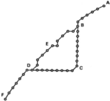
However, this measure of curvature defined at such a small length causes serious erroneous results. Fig. l shows a simple example of such cases where the problem is to find a smooth line connecting A and F. In the figure, values of points marked as o are one and the others are zero. The optimization method with the merit function defined in (5) finds a path A-B-C-0-F as the optimal solution, because sum of curvatures of this path is smaller than another path. However, we perceive another path A-B-E-D-F as more meaningful or good-shaped and the path B-C-D as the line caused by noise. This error has been caused by the very local measure of curvature defined only by three consecutive points. To avoid this problem, more global properties of the line defined over a wider range should be embedded into the merit function.
If the property of the line defined by a wider range, say k points, are embedded into the merit function, it becomes the form of
where all terms are functions of k variables. This is called a merit function of type k, and it is known that the required tables and computation time are exponetial with k to solve the problem with multistage optimization procedure.
,.S REPRESENTATION BY LINEAR SEGMENTS
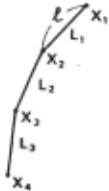
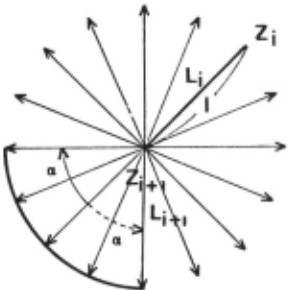
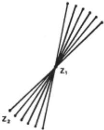
We have studied a different approach to avoid this difficulty, in which a line is represented by a sequence of connected linear segments Lt , LJ , ... , LN of length t instead of consecutive points , as shown in Fig. 2. Let us represent a linear segment L by an ordered pair of their endpoints ( Zt , Z2 ) and call z, the head and Z2 the tail of the segment. Then two linear segments L and L' are called connected if the tail of L coincides with the head of L'. If we call a connected linear segment of a segment L a successor of L, then each segment of length t has 27tt possible successors as shown in Fig. 3. However, since the line we want to detect are smooth ones, successors having curvatures less than a certain threshold m are considered as 'legal' successors. That is, if e ( z, , Z2 ) denotes the direction of the segment L ( Zt, z 2 ), then segments L' ( z't, z'2) having
are legal successors as shown in Fig. 3.
With this representation, a merit function to find a low-curvature curve having high gray levels in which the curvature is defined by the length of 2 t points can be given as
with the constraint defined in (8) , where g(Zt-t, Zt)is a mean of gray values of the points lying on the line L1-1 ( Zi- t , Zi ) . It will be noted that the problem of type 2 t if the curve is represented by a sequence of points is reduced to the problem of type 3 with this representation. Number of stages necessary to find a curve of N points is also reduced from . N stages with pointwise search to N/ t stages with this linewise search. Next, we will describe an algotithm to find optimal sequence of linear segments with respect to a given merit function.
Legal successors
Fig. 3. Legal successors of line L.
~.4 FINDING THE OPTIMAL SEQUENCE
For the sake of simplicity, let us first consider the problem of extracting from a picture a curve which starts in the first row and ends In the last row. First of all , for each admissible Zt , successors Z2 are determined with a constraint 1t~ e ( Zt , Z2 ) ~ 2 1t · Then , at the k-th stage , successors Zt+t are expanded for each admissible z" with the constraint 9 ( Zk-1 , Zk )- 9 ( Zt, Zu1 ) ~ !I where k=2, ... , N-1. For every value of Zt and zu1 ,
where h1 ( z1 , Z2 ) = g ( Z1 , Z2 ) and Ht-1 is the value of the output of the previous stages for all addmisslble Z~<,-1 . Then we obtain the maximal value of ht , Ht · wltn respect to Zt.-1 and the value of Zt-1 · Zt-1 · for which the maximum is achieved. These values · Ht and Zt-1 , are stored in the table for every value of Zt and Z~t.+l at each stage.
This process terminates at the N-th stage when some of the segments ( ZN-1 · ZN ) intersect with the last column. At this stage · the tail of each segment , ZN · which intersects with the last column is determined as the intersecting point of the segment ( ZN-1 · ZN ) and the last column. For every value of ZN-1 and ZN · we compute hN-1 defined in (10) and obtain the maximal value of hN-1 (ZN-1 · ZN). HN-i(ZN-1 , ZN). and the value of ZN-2 · ZN-2 · for which the maximum is achieved. Then · for all admissible ZN-1 · we compute the maximum of HN-I(ZN-1 · ZN)maximum of HN-1 ( ZN-1 , ZN ) with respect to ZN-1 and the value of ZN-1 . ZN-1 , for which the maximum is achieved. Finally, we obtain the maximal value of HN ( ZN-1 · ZN ) · M ( HN ) · and a value of ZN · ZN , for which the maximum is achieved. Then, tracing back the tables with the recursion formula defined in (4) , we obtain ZN · ZN-1 ,... · Z1 for which the maximum has been achieved.
2.5 LOCUS MODEL OF SEARCH
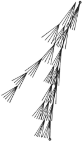
In order to decrease storage space and computation time, we introduce the locus model of search to this line finding system. In the multistage optimization process, all the paths generated during the optimization process are saved and evaluated until the last stage. However, it is usually not necesary to find the optimal path but it is sufficient to find good or near optimal solutions in practical applications. Therefore, we prune unpromising paths from the search tree at each stage. That is, after computing Ht at each stage, those paths having H" less than a certain threshold are not saved in the table; and therefore, their successors are not generated at the subsequent stages. Let us denote the maximum value of H" at the .k.-th stage as M( H" ), then the threshold is set as .t · M ( H" ) · 0 < .t < 1. This search method suppresses exponential growth of successors and only a beam of near-miss alternatives around the best path are retained as shown in Fig. 4.
J. FINDING A LINE WITH GIVEN KNOWLEDGE
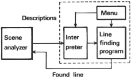
In this section, we will describe a line finding system which finds a globally good line with respect to the knowledge of the line given by the scene analyzer. A
variety of knowledge is available on the line to be sought. These various knowledge of the sought line must be easily expressed by and communicated to the line finder. The line finder consists of three components; a menu, a line finding program and an interpreter as shown in Fig. 5. The menu is a list of knowledge which can be utilized by the optimization process. Then the properties of the sought line can be expressed simply by descriptions which specify which items of the menu should be used in finding the line. The descriptions given by the scene analyzer are interpreted and embedded into the line finding program by the interpreter.
S.l MENU AIID INTERPRETER
The menu consists of properties of the line, some constraints on the line, constraints on the starting point, and terminating conditions, each of which is described below.
S.l.l PROPERTIES OF THE UN£
The menu for the properties of the line is listed in table I. The properties of the sought line are specified by the format (item, weight, parameter). For example, if we would like to find the low-curvature line of homogeneous gray level showing strong edgeness, then descriptions are given to the line finder as:
( HOMGRY k1 ),( EDGE k2 ),( LOWCURV k3 ). Then, these properties on the line are embedded into the merit function as follows:
f=klfl+k2f2+kJf3
S.l.~ SOIK£ CONSTRAINTS ON THE UNE
Constraints on the line which are difficult to embed in the merit function are given to the line finder as follows.
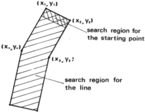
Search region: the expected location of the sought line is known using the relationship with th~ already found lines. This knowledge is given to the line finder as the search boundary of the line. The search boundary is given to the line firtder by a sequence of representative points as ( SEARCH ( x. , Y· ) ,( X2 , Y2 ) , ·.· ) . If the search boundary is given, a line is sought in the region bounded by the search boundary as shown in Fig. 6. This information greatly reduces the computation time and storage space, and increases reliability of the extracted line.
Length of linear segment t : we have four values for the length t ; 5, 10, 20, 30, and one of them can be specified considering the maximal curvature of the line to be sought. If it is not specified, length 20 is utilized.
Constraint on the successors m : the parameter m determines number of successors generated and is given considering the maximal curvature of the line to be sought. If it is not specified, 1 radian is used for Cl
Threshold .t : the threshold .t determines the width of the beam, that is a number of lines saved in the table at each stage. If .tis not given, 0.5 is used as .t .
| EDGE | Find a line having strong edgeness | _L e (Zt, Zt+t) |
|---|---|---|
| GVNGRY | Find a line having gray level G | _L g (Zt, ZuJ)- G |
| HOMGRY | Find a line having homogeneous gray levels | _L g (Zt-1, Zt)- g (Zt, Zt+J) |
| GVNDIR | Find a line having edge direction D | 2: d (z .... Zt-1) - D |
| HOMDIR | Find a line having homogeneous edge direction | _L d (Zt-1, Zt)- (Zt, Zt+J) |
| GVNSLP | Find a line having slope e | 2: e (zt, Zt+J)- e |
| LOWCURV | Find a low-curvature line | _L 8 (Zt-1, Zt)- 8 (Zt, Zt+J) |
| CONCURV | Find a constant-curvature line such as a circle | _L ( 8 (Zt-l, Zt-1) - 8 (Zt-1, Zt)) - ( (Zt-~o Zt) - e (Zt, zu.)) |
| GVNCURV | Find a line having the curvature C | 2: e (Zt. -•· z ... )- e (z .... zu•)- C |
E (z .... Zt+J)i mean value of edgeness of the segment (zt., Zt.+J)
G (Zt., Zt- J)i mean value of gray level of the segment (Zt., Zt+J)
D (z .... z .... ); mean value of edge direction of the segment (z .... z .... )
9 (z.,, Zk+J); slope of the segment (z ... z., ·· )
8.1.8 CONSTRAINTS ON THE STARTING POilfTS
Selection of the starting points of the line is very important to reduce growth of successors in subsequent stages. We have two constraints on selecting the starting point; 1) search boundary for the starting points and 2) properties of the starting point. In many cases, more restricted search boundary is available for the starting point than for the sought line. This search boundary is given to the line finder by a sequence of representative points as
- If a search boundary is given, the starting point is sought in the region bounded by the search boundary. If it is not given, the search boundary for the line is utilized.
Properties of the starting point listed on the menu are gray level, edgeness and edge direction. The properties on the starting point is given in the similar manner to the line. For example, if we would like to find the points having strong edgeness and edge direction D with weights k.1 and k1 respectively, then the following descriptions are given:
( SEDGE k.1 ),( SDIREC k.2 D ).
Then the following merit function is generated by the interpreter:
Then, the promising points are selected with respect to the merit function for the starting point in the search region.
8.1.4 T£RJKINATING CONDITIONS
There are four terminating conditions in line following as follows.
- Line segments of the current stage intersect with line segments of the first stage. This terminating condition is used when the sought line is closed.
- Line segments of the current stage intersect with the other lines which are already found in the picture.
- Line segments of the current stage intersect with the line L specified as the terminating one.
- There is no promising line segment at the current stage. That is, score of the best line segment at the current stage M1< is much smaller than the score of the best line segment of the last stage Mk-1, such as· Mt ~ ~ M .. -1 where~ < 1.
If we would like to use the terminating conditions, for example 1 and 4, then the descriptions are given to the line finder as follows;
where ~ is a threshold.
8.2 LIN£ FINDING PROGRAM
When the descriptions on the sought curve are given, these are interpreted and embedded into the line
- finding program by the interpreter as described before. Then the line finding program seeks a globally good line with respect to the given knowledge as follows.
- Compute the value of merit function f( Z1 ) for every point Z1 in the search region for the starting point, and select promising starting points. Let us denote the r.1.aximum of f( Z1 ) as M (f( Z1' )), then those points having value of f( Z1 ) larger than
- T·M(f(ZI )) are selected as promising starting points.
- At the first stage, determine successors Z1 for each selected points Z1 and select promising ones among Z1. For each selected point Z1 , its successors Z2 are determined with the constraint that Z2 must be in the search region for the line , and the merit function f(z1. z1) are computed. Then those seyments having f(zl , z2) larger than .t·M(f( z1 , Z1 ) ) are selected as promising ones. If the search region for the starting point is given around the middle of the sought line, then two beams are obtained as shown in Fig. 7. In this case, one of them is followed first.
- At the k.-th stage, determine the successors Zu1 for each z., and select promising ones among Zu1. For each z.. , its successors are determined with constraints that Zu1 must be in the search region and e ( Zk-1 , Zk )- e ( Zk , Zu1 ) ~ Clo If the given merit function is type i (2 ~ i ~ 4 ), then we compute
for every value of Zk-1+2 , ... , Zu1. We obtain the maximal value of h., , H., , with respect to Zk-Hl and the value of Zk.-1+2 , Zk-1+2 , for which the maximum is achieved , for every value of Zt-IH , ... , Zt.+1. Let us denote the maximum of H., as M ( H., ). Then, those points Zk+l having H., larger than .t·M ( H., ) are selected as promising points. The value of H., and Zt-1+2 of the promising points z .. are saved in the table.
- Check the terminating conditions. If one of the terminating conditions specified by the descriptions is satisfied, then the line following is terminated. At this last stage, the tail of each segment ZN is determined as the intersecting point of the segment (ZN - 1, z.,.) and the line specified by the terminating conditions.
- Try to follow the other end of the line using the above-mentioned procedure , with ( Z2 , z, ) as the starting line segments. When both sides terminate, then obtain the maximal value of the merit function, and a sequence of line segments for which the maximum is achieved by tracing back the tables.
4. EXPERIMENTAL RESULTS
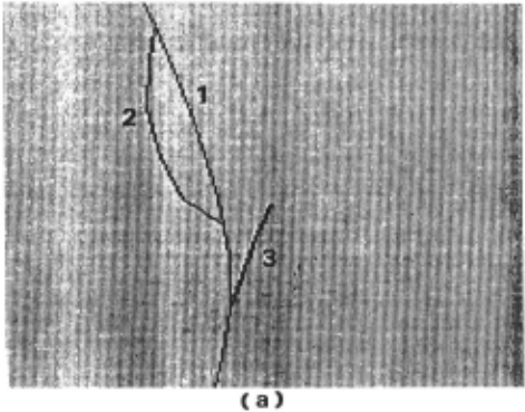
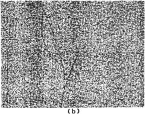
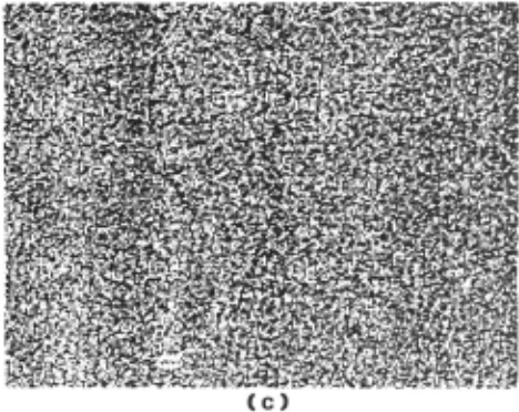
The proposed line finding system was implemented in Fortarn IV on a HP-2108 computer and was utilized for analysis of heart walls, blood vessels and complex industrial parts. We show a result on the test image shown in Fig. 8(a) by adding different amount of noise to the image. The image consists of 256 by 256 points, each point having 16 levels of gray. Our purpose is to detect smooth line 1 in the presence of noisy lines 2 and 3. In the image, the gray levels of the lines 1, 2 and 3 are 10, 11 and 12 respectively and the gray level of the background is 5. In Fig. 8 (b) and (c), independent amount of noise is added to every point. The statistical distribution of the noise at every point is normal, with mean value zero and standard deviation 4 and 6, respectively. Note that the line is recognizable in Fig. 8(b) but quite unrecognizable in Fig. 8(c).
The knowledge available of the curve is smooth, has large value of gray, starts in the first row and ends in the last row. Therefore, the descriptions given to the line finding system are as follows: (EDGE 1), (LOWCURV 5), (SSERCH (1,1),(256,1)) (TERM 3 (1,256),(256,256))
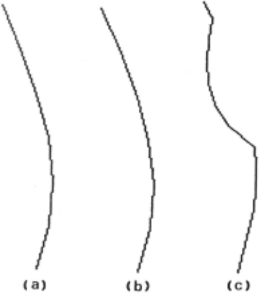
Fig. 9(a) and (b) show the results for the image!' of Fig. 8(b) and (c). It will be noted that the line is detected correctly even in the presence of heavy noise. If the second description is eliminated, that is the low-curvature is not utilized, then the pass 2 is selected as shown in Fig. 9(c) which is the result for the image of Fig. 8(b) .
5. CONCLUSION
We have presented a line finding system that can detect a globally good line with respect to the given knowledge of the line. The proposed method Is very efficient since I) size of tables required at each stage and number of stages is greatly reduced by representing a line by a sequence of linear segments, 2) a locus model of search is utilized to supress the exponential growth of search trees, and 3) several constraints available of the sought line are utilized to limit search space or growth of successors, such as search boundary, constraints on the starting point, etc.
The length of linear segment l seriously affects computational efficiency. Therefore, if the sought curve is smooth and can be approximated by long linear segments, then large value should be given to t . On the contrary, if small variations on the line is important or the sought line has high curvature, then small value must be given to l . However, it is more efficient that we first obtain an approximate line with large t and then obtain more details with small t in the neighborhoods of the approximated line than obtaining the line with small t from the beginning.
We have used a locus model of search instead of the best fi rst search of A· algorithm for obtaining sub-optimal solution. The reason of this selection is that its control structure is simpler than the A· algorithm and it is easier to understand the behavior of search process since the locus model does not need backtracking. Another reason which is more important is that it permits parallel computation of all the linear segments at every stage.
In this system, it is very easy to communicate the knowledge of the sought line to the line finder since a variety of knowledge can be expressed simply in the form of descriptions. The menu provided in the system is sufficient for our current tasks. However, it is easy to change the menu if it is necessary.
We have applied the proposed method for a variety of scene analysis tasks and the results have shown the effectiveness of the proposed method to find a globally good line with respect to the given knowledge. However, for complex scenes where many kinds of objects exist and a priori knowledge on the scene is not available, we must first extract distinct lines as initial information on the scene to select possible models of objects in the scene. For this purpose of extracting initial information, there exist several methods such as planning[ 6] , detection of distinct edges[ 7] and extended Hough trans formation[&]. The proposed line finder is then used to find subtle lines using knowledge of the objects and their contextual relations.
REFERENCE
[ 1] A. Martelli : An Appllcation of Heuristic Search Methods to Edge and Contour Detection, Commu. ACM 19, pp. 73-83, 1976.
- U . Montanari : On the Optimum Detection of Curves in Noisy Pictures, Commu. ACM 14, pp. 335-345, 1971.
- [3) A. Martelli : Edge Detection Using Heuristic Search Methods, Comput. Grap. Image Proc. 1, pp. 169-182, 1972.
- S.M. Rubin and R. Reddy: The Locus Model of Search and Its Use in Image Interpretation, Proc. 5th IJCAI, pp. 590-595, 1977.
- M. Yachida and S. Tsuji : A Versatile Machine Vision System for Complex Industrial Parts , IEEE Trans. C-26, pp. 881-894, 1977.
- f6] M. D. Kelly : Edge Detection in Pictures by Computer Using Planning, in Machine Intelligence, 6, pp. 379-409, 1971.
- A. K. Griffith : Edge Detection in Simple Scenes Using a Priori Information, IEEE Trans. C-22, pp. 371-381, 1973.
[8] S. Tsuji and F. Matsumoto: Detection of Ellipses by a Modified Hough Transformation, IEEE Trans. C-27, pp. 777-781, 1978.
@inproceedings{ijcai1979p215,
  title     = {A Knowledge Directed Line Finder for Analysis of Complex Scenes},
  author    = {Yachida, Masahiko and Ikeda, Motozo and Tsuji, Saburo},
  booktitle = {Proceedings of the Sixth International Joint Conference on
               Artificial Intelligence, {IJCAI-79}},
  publisher = {International Joint Conferences on Artificial Intelligence},
  editor    = {Bruce G. Buchanan},
  year      = {1979},
  month     = {8},
  url       = {https://ijcai.org/proceedings/1979/215},
}
TY - CPAPER TI - A Knowledge Directed Line Finder for Analysis of Complex Scenes AU - Yachida, Masahiko AU - Ikeda, Motozo AU - Tsuji, Saburo T2 - Proceedings of the Sixth International Joint Conference on Artificial Intelligence, IJCAI-79 PB - International Joint Conferences on Artificial Intelligence PY - 1979 UR - https://ijcai.org/proceedings/1979/215 ER -Copied
Machine-readable versions of this paper, for tools and AI agents:





