
A Formal Description for Two-Dimensional Patterns
Proceedings of the First International Joint Conference on Artificial Intelligence. Linguistic and Contextual Methods in Pattern Recognition. Pages 621-628.
© 1969 International Joint Conferences on Artificial Intelligence
Abstract
A "structural description" for two-dimensional black and white patterns is defined as the set of contour lines for an appropriate function which fits the binary pattern. These contour lines are mutually nonintersecting closed polygonal curves with edges in only eight different directions and they represent the boundari e s between connected black and white areas of the pattern. Rigorous procedures are described to transform a "matrix pattern" into a "structural description" and vice versa. Advantages of this method for describing patterns previous to pattern recognition are discussed at some length.
- C. T. Zahn, "Two-dimensional pattern description and recognition via curvaturepoints," Report No. SLAC-70, Stanford Linear Accelerator Center, Stanford University, Stanford, California (1966).
- R. Courant and H. Robbins, What is Mathematics? (Oxford University Press, London, 1941); pp. 267- 269.
- L. Uhr, "Pattern recognition," in Pattern Recogni- tion, ed. Leonard Uhr (John Wiley & Sons, New York, 1966); pp. 365-381.
- F. Attneave, "Physical determinants of the judged complexity of shapes, " J. Exptl. Psychol. 53, 221 (1957). -
- J. Y. Lettvin, H. R. Maturana, W. S. McCulloch and W. H. Pitts, "What the frog's eye tells the frog's brain," Proc. IRE 47, (November 1959); pp. 1940-1951.
- D. H. Rubel and T. N. Wiesel, "Receptive fields, binocular interaction, and functional architecture in the eat's visual cortex," J. Physiol. 160, 106 (1962). -
- R. S. Ledley, "High-speed automatic analysis of biomedical pictures," Science 146, 216 (1964).
- A. C. Shaw, "The formal description and parsing of pictures, Report No. SLAC-84, Stanford Linear Accelerator Center, Stanford University, Stanford California (1968).
- H. Freeman, "On the encoding of arbitrary geo- metric configurations, " IRE Trans. on Electronic Computers EC-10, (1961); pp. 260-268.
References were extracted automatically from the PDF and may contain errors.
Full text extracted automatically from the PDF; figures, tables and equations may differ. The PDF is the version of record.
Introduction
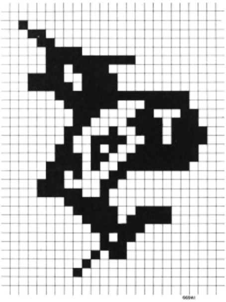
This paper presents a method for obtaining a "struc tural description" of any two-dimensional picture whose e lements are a finite set of points in the plane each hav ing value zero (white) or one (black) and such that the points are arranged in the form of a square lattice. Figure 1 shows one such picture. The "structural
C. T. Zahn
Stanford Linear Accelerator Center Stanford University, Stanford, California
description" we employ consists of a set of simple polyg onal closed curves whose vertices are ordered in either clockwise or counter-clockwise sense. These curves represent the continuous boundaries between connected sets of black points which we call "objects" and con nected sets of white points which we call "holes. " Fig. 2 depicts the structural description of the pattern in
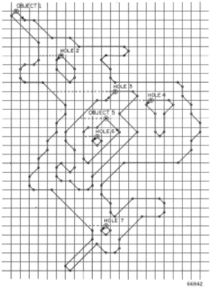
Fig. 1. Our structure also includes information indi cating which curves are inside each other as shown schematically by dotted lines in Fig. 2. The points of a curve are ordered so that the curve is traced keeping black points to the right and white to the left. As a result, curves which define the outside boundary of black areas (objects) proceed clockwise and those for white areas (holes) proceed counter-clockwise . It should be noticed that the curves do not go through the outermost picture points of an area but rather go be tween these outermost points and the adjacent points of opposite color.
Our selection of this particular format to describe the information content of a black/white pattern was motivated by a belief that the sequential trace of the boundary of an object contains the most useful data for recognizing objects one from another in a great many appli cations. Experimental evidence from the psychology of hu man visual perception and the neurophysiology of animal visual perception support this beliefto an amazing extent.
For a more detailed description of this "structural description" and an extended discussion of its uses, the reader is referred to Zahn. 1
Structural Description as Contour
The closed curves of the "structural description" are, in fact, the contour lines at a height of 1/2 for a continuous function F(x, y) defined over the square area of the picture and such that F takes value 1 where the picture has a black point and 0 where it has a white point. The precise construction of F is as follows:
Consider the subdivision of the picture area into smaller squares defined by the square matrix of picture points by drawing horizontal and vertical lines through the points of the picture. It should be clear that a tri angulation* of the picture area can now be effected by separately triangulating each smaller square, as shown in Fig. 3. We shall describe rules for determining which diagonal will be added to each square to complete the triangulation.
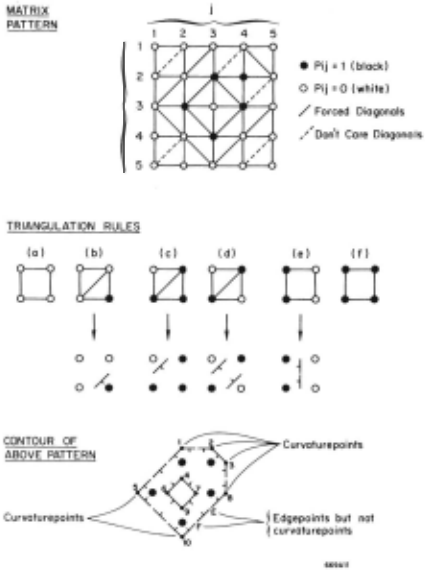
In deciding how to triangulate the square mesh we follow two simple rules. If there is a choice of whether to connect two black points or two white points, choose the black and try to have as few curvaturepoints as possible. The triangulation rule embodied in (d) of Fig. 3 assures that black points have precedence, while rules (b) and (c) prevent a straight edge at 450 from being encoded as a saw-tooth contour line . . ·The reader may verify these statements by choosing the other diag onal and then constructing the contour . The actual con tour for the top pattern in Fig. 3 is presented at the bottom of Fig. 3 and hatch marks have been appended to show which side of a contour line is the high or black side.
*Subdivision of plane area into disjoint triangles.
There are only six essentially different combina tions of values possible for the corners of a square. These are shown in Fig. 3 along with the proper diag onal. Where no diagonal is shown it means that either one may be chosen.
Now that the picture area has been triangulated, we define our function F separately for each triangle. Supposing some triangle to have vertices A, B, and C, we let P A· PB, Pc denote the picture values at points A, B, C whicli are indeed points of the "matrix picture . " There is a unique linear function F*(x, y) = ax+ by+ c which takes on values P A· PB, Pc at points A, B, C. Each triangle of the triangulation determines uniquely an FABC and F is defined so that F(x, y) = FABC(x, y) whenever (x, y) is inside or on triangle ABC.
The proofs that F is well-defined and continuous are easily derived from the exemplary behavior of linear functions. In fact, the only way discontinuity could pos sibly occur is by way of F being double defined for some point on a common edge AB between two triangles tl1 and t.2. The reason that this cannot occur is because Fi and F2 (the linear functions for tl1 and t. 2 ) when restricted to the edge AB are both found to vary linearly between A and B and to have the same values at these two points; hence Fi = F~ on the edge AB and F is well defined.
Having defined F over the picture area as a contin uous piecewise-linear approximation to the original pic ture, we can simply repeat that the "structural descrip tion" of the picture is the set of contour lines of F drawn at a height of 1/2. This approach certainly corresponds well with any intuitive notion of edges in a binary picture.
Curvaturepoints
We use the term "curvaturepoints" to describe the points where the contour lines (called "edges") change direction. For example, in the bottom of Fig. 3 the numbered points 1 - 10 are the curvaturepoints whereas E and F are points on the contour but not at bends. This is because the two sections of contour line which meet atE are both in the same direction. t Referring to Fig. 4, we see that at E there is an incoming edge and an outgoing edge both in direction 5, whereas at point 8 there is an incoming edge in direction 6 and an outgoing edge in direction 5 .
It turns out that curvaturepoints can only occur at points midway between two picture points. Further more, the question of whether or not a given point is a curvaturepoint can be determined by referring to the values of just 6 picture points arranged in a (2 x 3) or ( 3 x 2) array. Figure 4 depicts how curvaturepoint 4 of Fig. 3 is determined by the (2 x 3) window shown. If Pij denotes the value of picture point (i, j) then (P33 = 0, P23 = 1 and P 34 = 1) implies that there is an inco~ing edge in dire.ctiOI~ 3; further~ore (P 33 = ~· P 23 - 1 and P 32 = 1) 1mphes an outgomg edge m direc tion 5. As a result, we record that the fourth curva turepoint is at i = 2. 5, j = 3 with EDGEIN = 3 and EDGEOUT = 5.
tContours are directed so that the hatch mark is on the right.
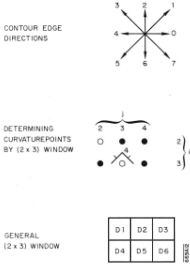
If D 1 - D 6 denote the picture point values as shown in Fig. 2, then the following hold for the point midway between D2 and D5:
First of all, the point is an edgepoint if and only if D2 and D5 are different in value. If not, it is useless to proceed further with this point. The values EDGEIN and EDGEOUT are determined by the following logic formulas, which are easily implemented by digital hard ware:
| D5 = 1, D1 = D2 | = D4 = 0- EDGEIN = 1 |
| D2 .= D6 = 1, D5 = 0 | -EDGEIN = 3 |
| D2 = D3 = 1, D5 = | D6 = 0 -EDGEIN = 4 |
| D2 = 1, D3 = D5 = | D6 = 0-EDGEIN = 5 |
| D1=D5=1,D2=0 | -EDGEIN=7 |
| D4 = D5 = 1, | D1 = D2 = 0- EDGEIN = 0 |
| D3 = D5 = 1, D2 = 0 | -EDGEOUT = 1 |
| D2 = 1, D1 =D4 =D5 = 0 | -EDGEOUT = 3 |
| D1 =D2 = 1, D4 =D5 | = 0 -EDGEOUT = 4 |
| D2 = D4 = 1, D5 = 0 | -EDGEOUT = 5 |
| D5 = 1, D2 = D3 = D6 = | 0- EDGEOUT = 7 |
| D5 = D6 = 1, D2 = D3 = | 0- EDGEOUT = 0 |
The determination of which edgepoints are curva turepoints is then simply a matter of whether or not EDGEIN F EDGEOUT. It should be fairly clear from the simplicity of the above conditions that the digital logic involved is easily implemented.
Linkage of Curvaturepoints
So far we have described how an input "matrix pic ture" can be transformed into a set of "curvaturepoints" of its approximate contour lines. It is still not entirely obvious that these separate and sometimes widely scat tered points can be linked together in the proper way to reconstruct the polygonal curves of its "structural de scription." The reader may have noticed that in an earlier section we spoke of the "structural description" as consisting of closed curves, whereas it is perfectly possible for contour lines to end at the edge of a map or in our case, a picture. To eliminate any chance of confusion, we shall assume that the picture points on the boundary of an input picture are all zero. This will force all contours to be closed curves but will not really hamper the validity of our approach. The only reason we make this assumption is to simplify the discussion below; in practice there is no need to border a picture with zeros this way, but the linkage of curvaturepoints is somewhat more complicated otherwise.
We shall assume that all the curvaturepoints of a given input picture are delivered to a general purpose digital computer in the order in which they are encoun tered during a normal left-to-right and top-to-bottom raster scan. The rows will be designated by increasing values of Y and the column positions within each row by increasing values of X. Also, the incoming and out going edge directions EDGEIN and EDGEOUT are con sidered an integral part of any curvaturepoint. For example, the simple pattern of Fig. 3 would be repre sented as:
| POINT | y | X | EDGE IN | EDGEOUT |
|---|---|---|---|---|
| (1) | 1.5 | 3.0 | 1 | 0 |
| (2) | 1.5 | 4.0 | 0 | 7 |
| (3) | 2.0 | 4.5 | 7 | 6 |
| (4) | 2.5 | 3.0 | 3 | 5 |
| (5) | 3.0 | 1.5 | 3 | 1 |
| (6) | 3.0 | 2.5 | 5 | 7 |
| (7) | 3.0 | 3.5 | 1 | 3 |
| (8) | 3.0 | 4.5 | 6 | 5 |
| (9) | 3.5 | 3.0 | 7 | 1 |
| (10) | 4.5 | 3.0 | 5 | 3 |
A simple inspection of the above table shows the following interesting facts about the two POINTS 1 and 5. First of all, EDGEIN [ 1] = EDGEOUT [ 5] = 1 and X [ 1] + Y [ 1] = X [ 5] + Y [ 5] = 4. 5; furthermore, there is no curvaturepoint P between* these two which satis fies the condition X[ P] + Y[ P] = 4. 5. It should be clear that whenever two points P and Q (P < Q) have the same value of X + Y, then they lie on the same line drawn in direction 1- 5 (see Fig. 4). If, in addition, there is no intermediate curvaturepoint and either EDGEIN [ P] = EDGE OUT [ Q] = 1 or EDGEOUT [ P] = EDGEIN [ Q] = 5, then the two points are adjacent curvaturepoints of the same contour curve and hence should be linked together. There are similar conditions for the linkage of points with the same (X- Y), X or Y values. Each case is associated with a pair of direc tions (respectively 3-7, 2- 6 or 0- 4) and the precise conditions are geometrically self-evident. These con ditions are all that are needed to perform the linkage of the curvaturepoints into simple closed polygonal curves. The implementation of this procedure uses very strongly the fact that the points are ordered by in creasing X within increasing Y since there is a great deal of geometric information implicit in this sorting order.
The data structure required to implement the link age of curvaturepoints is essentially a cyclic list; this requirement reflects the natural structure of a closed polygonal curve as well as the fact that at various times during linkage we are required to join together two al ready created partial polygonal curves. This joining (concantenation) would be quite difficult if simple arrays were used. ·
Smoothing Curves
In Fig. 5, we have redrawn the outermost curve of the "structural description" in Fig. 2. Some of the curvaturepoints are not solid dots and these are to be deleted from the description. The criteria which con trol which points will remain are explained below, along with an intuitive justification for performing this smooth ing operation.
An "inflection" will be defined as two adjacent cur vaturepoints, one with a bendt of -1, the other+ 1, and such that the distance between the two points is 1 or 12. Referring to Fig. 5, the pair of points (3,4) are at dis tance 1 from each other and have bends respectively+ 1 and -1 as shown in the insert. As a result, the incom ing edge at 3 and the outgoing edge at 4 are in the same direction, namely 7. Similarly the pair (6, 8) are at distance v'2 with bends -1 and+ 1; hence, we have an other "inflection."
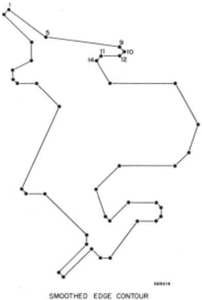
When points 3, 4, 6 and 8 have been deleted, the sequence of curvaturepoints becomes 1, 5, 9, ... and point 5 retains a bend value of + 1. Since we allow point deletions to occur only in pairs with bends that cancel (+ 1 and - 1), it is clear that the total bend around a
*meaning a point with a number between 1 and 5.
tThe bend at any curvaturepoint measures the change in direction of the edge at that point in units of 45°. Bends toward the right are negative and toward the left, pos itive.
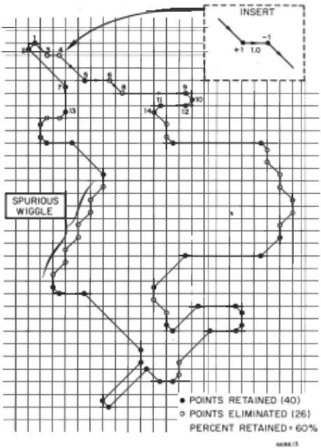
curve is not disturbed at all. The bend at point 5 in Fig. 6 is not exactly+ 1 as can readily be seen, but as an approximation it does not really go far wrong. Fur thermore, if more precision is required, it can be cal culated from the X and Y coordinate values of the· 3 points 1, 5 and 9.
The main advantages of performing this smoothing of inflections are the reduction in the amount of data to be processed in subsequent discrimination algorithms and the elimination of some sequences of edge bends which we may call "spurious wiggles" since the cor responding edge in a typical original continuous pattern was probably straight. Figure 5 shows a "spurious wiggle" of 4 pairs of points. In the example depicted the reduction in data is substantial, amounting to 40%, although the picture pattern contains a great deal of real detail.
As a final point we want to make it perfectly clear that this smoothing procedure is not an absolutely nec essary part of the overall method. Depending on the particular application, it may or may not be appropri ate. We present it here in place of several other smoothing algorithms which we have experimented with because it has been found to accomplish a substantial reduction in data without eliminating many major de tails and while requiring only simple decision criteria.
Bend Groups
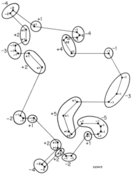
When the sequence of curvaturepoints describing a single closed contour has been constructed and the "in flections" have been deleted as described in the previous section,. then a very compact but extremely character izing signature can be computed by merging curvature points according to the following rules:
Transform the closed curve into a sequence of in tegers representing amounts of bend by adding together the values of bend for two adjacent curvaturepoints of like sign whenever their distance apart is less than some threshold which is appropriate to a given application.
Figure 7 depicts how the grouping of like points would be made for our sample curve of the last section, assuming a threshold distance of approximately 4. 0. The compact signature for this curve is (-4, +1, -4, +4, -1, -3, +5, -5, +1, -2, +2, -4, +2, +1, -2, +2, -3, +2).
Once· again we must emphasize that special appli cations will generally suggest variations in the merging of bends in addition to guiding the determination of the distance threshold. Some applications may, of course, require the retention of more detailed edge length infor mation in which case this simple scheme would not be appropriate.
Recovery Algorithm
An important property of "structural descriptions" is that an algorithm exists which will recover the orig inal digitized binary matrix pattern given only the struc tural description. We shall give a brief outline of such an algorithm and discuss the theoretical foundation for its validity.
The famous mathematical theorem known as the "Jordan Curve Theorem" states that any simple closed curve in the plane divides the remainder of the plane into two distinct sets called the "inside" and "outside," such that any two points in the same set can always be connected with a continuous curve lying entirely in that same set; any continuous plane curve joining a point "inside" the curve to one "outside" must have at least one point in common with the closed curve. The proof of this theorem is much simpler for polygons than for general curves; Courant and Robbins2 give a proof for the polygonal case which depends on the fact that if a point "outside" a closed curve r is connected by a straight line L to another point P, then P is also "out side" T if and only if L intersects T an even number of times. If L intersects T an odd number of times, then p is "inside" r.
The algorithm we propose is based on the latter fact, which is also proved in Ref. 2. Referring to Fig. 9, we shall show how it is possible to determine that the points in ranges {3 and 8 (for X = X 0 ) are inside r while ranges a, y and E are outside. The proper assignment of values then depends only on the status of r ("object" or "hole").
The determination that ranges {J and o are inside r proceeds as follows:
Curve r is traced from its top all the way around and back to the top again. Whenever the curve r crosses the vertical line X= x 0 , we record the fact by making a mark in all points below the crossing. For example, r crosses first at e 1 and all points in ranges, {J, y , a and E are marked + as shown in the table. This means that each of these marked points can be con nected by a straight line to the top of the picture area only by a line crossing r at e 1 . The table is filled in for e 2 , e 3 , and e 4 in an entirely similar manner. After e4, there are no more crossings and the curve returns to the starting point. We then determine which points have received an odd number of marks and find that all points of ranges {J and 0 are inside r.
When this procedure is carried out for all vertical lines x 0 , then the "inside" points for r will have been determined. In any actual implementation, we assume that all Xo's would be handled simultaneously while r was being traced only once.
If the same process is repeated for all curves r in a "structural description" then the result is just as valid as for one curve because curve crossings always repre sent a color change.
No claim is made for the efficiency of this procedure; we merely wanted to show with some degree of mathe matical rigor that the "structural description" contains all the information of the original digitized pattern and it can be mechanically recovered if necessary.
Advantages of the Curvaturepoint Method
The generality of the curvaturepoint method is one of its most important properties. The method applies to any "black and white" pattern whose significant content consists of connected sets of similar points. Hence, it also applies to input pictures which can be made to com ply with this condition by suitable preprocessing; fairly simple local transformations on binary pictures have been found to be very successful at r egularizing pictures in this way. Our method can be used in some cases to extract contrast information from grey-scale* pictures by converting the picture to binary several times using differ ent thresholds. This idea is more fully elaborated in Zahn.1 This applicability to multilevel pictures should come as no surprise when it is remembered that the method is simply a contouring of a two-dimensional distribution of numerical values .
Simplicity and mathematical rigor are properties of the method which we feel have been largely overlooked in most "edge-detection" schemes. The two properties are closely related, for the mathematical rigor with which "curvaturepoint extraction" and "linkage" are performed is a direct consequence of the simple and straightforward definition of the "structural description. " Being contour lines of a simple function, the "structural description" is constrained to consist of non-intersecting closed polygonal curves whose edges are directed in only eight different ways and whose edge bends or "curvaturepoints" are also tightly constrained. It is precisely because of such constraints that the "linkage" of widely .spaced "curvaturepoints" can be accomplished in a completely assured way. Not only is the transformation from bin ary pattern to structural description rigorous and uniquely defined; the reverse transformation (see Re covery Algorithm) exists as well, proving a unique one to-one correspondence between a binary pattern and its structural description and also showing that the struc tural description contains total information from the binary pattern.
*Picture values range over an ordered finite set such as (0, 1, 2, 3).
One of the most serious obstacles to the further development of digital picture processing is the volume of data implied by the two-dimensionality of pictures. When the resolution is doubled the data volume is quad rupled; a picture 1, 000 x 1, 000 has one million data points, an amount which is still prohibitively high for even the largest computers. The "structural descrip tion" on the other hand contains one-dimensional infor mation (contour lines) and therefore the data volume increases only linearly with resolution. This means that if "curvaturepoint extraction" can be done in special digital hardware then the storage requirement for imple menting the method on a general purpose computer will be greatly reduced and more richly detailed patterns can be handled. The "linkage" would be accomplished by programming. It turns out very happily that "curvature point extraction" is defined by extremely simple Boolean logic (see Curvaturepoints) and its digital hardware implementation could be accomplished with the addition of two long shift registers. We consider this efficient implementation to be an extremely vital aspect of the method.
The intuitive character of our method should prove of considerable benefit in constructing recognition al gorithms. In a recent article Uhr3 claims that edges , angles and the interrelations between lengths and slopes are the important and meaningful properties for human pattern perception and recognition. If this is true then it is reasonable to expect that algorithms based on "structural descriptions" will be highly intuitive in na ture and hence less mysterious than those based on in formation other than edges. In support of Uhr's claim we shall cite evidence from psychology and neurophysi ology which tends to indicate the predominance of edge information in animal visual perception. Attneave4 in experiments on human subjects found that the number of bends in polygonal shaped objects accounted for 80% of the difference between objects when rated by subjects according to judged complexity. This clearly suggests importance of curvaturepoints. Other researchers have found that an object's visibility is related to the length of its boundary, strongly suggesting that for purposes of perception the edge is the predominant information con tent.
The research of Lettvin et al. 5 on the optic nerve cells in the frog indicates thatsignals reaching the frog's brain from its eyes are highly contrast-oriented. Hubel and Wiesel6 determined that nerve cells in the cat' s brain are specific to the existence of edges in the visual field of given slope. This neurophysiological evidence if extrapolated to the human case lends further support to the claim that edge information is the raw data for visual perception mechanisms in man.
Although the method is clearly directed toward rec ognition via edge-bend-sequence, nevertheless familiar quantitative properties such as perimeter, area, mo ments, height and width are easily calculated. In addi tion, we can define and compute reasonably intuitive quantitative measures of oblongness, compactness, wigglyness and total absolute curvature.
For some pattern recognition applications (character recognition especially) it is useful to have a method which is position and size invariant. "Structural de scriptions" contain position and size information but in such a way that it is quite easily disregarded. Rotation invariance is also easy to achieve by simply considering the sequence of curvaturepoints without paying attention to the initial edge direction. The information is always there when needed, however, so that recognition methods sensitive to position, size and rotation are not hampered in the least.
A pattern description method is greatly enhanced if it is compatible with some fairly elegant language for pictures. This is particularly true if the language has a formal phrase structure grammar which allows pat tern recognition to be accomplished by the formal par sing procedures which have been developed for such grammars. The survey paper of Miller and Shaw13 discusses this aspect of picture processing quite com prehensively. Ledley7 for example, has shown that formal parsing techniques can be used to recognize dif ferent chromosome shapes by transforming their edge sequences into a string of primitives and then parsing this string. For example, in Fig. 8 0 means no bend, E means sharp 180° convexity, Y means sharp 1800 con cavity, etc. These are the primitives of the language. The formal grammar would define "arm" as OEO, "double arm" as armY arm, etc.
An essentially one-dimensional data format seems to be advantageous for linguistic processing of pictures because phrase-structure grammars describe sets of "strings." When the data is not in a "string" format there are some subtleties involved in making the cor respondence between the data and linguistic formalism. The recent work of Shaw8 shows that automatic parsing recognizers can be quickly implemented when the struc ture of the picture can be represented by a suitable one dimensional grammar. Syntax directed parsing methods are employed so that new recognition tasks require only a new syntax table and specially written primitive rec ognizers.
In addition to formal language parsing methods, our "structural description" can be used very readily in a decision tree approach to recognition. In fact, the cyclic list data format of the "structural description" lends it self naturally to sequential decisions made as the list is traversed. As with all pattern description schemes, it is possible to reduce to a vector of quantifiable proper ties and then use one of the many procedures based on the property vector representation of a pattern. The algorithms of Freeman9, 10, 11 for "curve segment matching" are applicable with almost no change since "structural descriptions" are essentially "Freeman encodings" of the curves defining boundaries in a binary picture. For example, the Freeman chain-encoding of the closed curves of Fig. 3 would be (00766555333111) and (5713). Each digit represents a unit vector as shown in Fig. 4 and the curve is traced sequentially. Our "structural descriptions" vary from this format only to the extent of merging like-direction contiguous unit vectors into a single vector with length. The "structural description" for the outer curve of Fig. 3 is essentially (0, 2; 7, 1; 6, 2; 5, 3; 3, 3; 1, 3). These curve matching algorithms are capable12 of putting together an "apictorial jigsaw puzzle" which attests to the sub tlety of their shape discrimination.
Acknowledgements
The author would like to thank Alan Shaw of Cornell University* and Jeno Gazdag of IBM for many hours of very useful discussion on pattern recognition methods; Robert H. Penny of General Electric Co. for introducing us to and stimulating our interest in digital picture processing and William F. Miller of Stanford Univer:sity for his continuing encouragement and support of this research. We also thank the referee for several con structive suggestions.
@inproceedings{ijcai1969p54,
  title     = {A Formal Description for Two-Dimensional Patterns},
  author    = {Jr., Charles T. Zahn},
  booktitle = {Proceedings of the First International Joint Conference on
               Artificial Intelligence, {IJCAI-69}},
  publisher = {International Joint Conferences on Artificial Intelligence},
  editor    = {Donald E. Walker and Lewis M. Norton},
  pages     = {621--628},
  year      = {1969},
  month     = {5},
  note      = {Linguistic and Contextual Methods in Pattern Recognition},
  url       = {https://ijcai.org/proceedings/1969/54},
}
TY - CPAPER TI - A Formal Description for Two-Dimensional Patterns AU - Jr., Charles T. Zahn T2 - Proceedings of the First International Joint Conference on Artificial Intelligence, IJCAI-69 PB - International Joint Conferences on Artificial Intelligence PY - 1969 SP - 621 EP - 628 UR - https://ijcai.org/proceedings/1969/54 ER -Copied
Machine-readable versions of this paper, for tools and AI agents:





