
Relation-Based Counterfactual Explanations for Bayesian Network Classifiers
Proceedings of the Twenty-Ninth International Joint Conference on Artificial Intelligence. Main track. Pages 451-457.
https://doi.org/10.24963/ijcai.2020/63
Keywords
- Uncertainty in AI: Bayesian Networks
- AI Ethics: Explainability
Abstract
We propose a general method for generating counterfactual explanations (CFXs) for a range of Bayesian Network Classifiers (BCs), e.g. single- or multi-label, binary or multidimensional. We focus on explanations built from relations of (critical and potential) influence between variables, indicating the reasons for classifications, rather than any probabilistic information. We show by means of a theoretical analysis of CFXs’ properties that they serve the purpose of indicating (potentially) pivotal factors in the classification process, whose absence would give rise to different classifications. We then prove empirically for various BCs that CFXs provide useful information in real world settings, e.g. when race plays a part in parole violation prediction, and show that they have inherent advantages over existing explanation methods in the literature.
- [Bach et al., 2015] Sebastian Bach, Alexander Binder, Grégoire Montavon, Frederick Klauschen, Klaus-Robert Müller, and Wojciech Samek. On pixel-wise explanations for non-linear classifier decisions by layer-wise relevance propagation. PLOS ONE, 10(7):1-46, 07 2015.
- [Bau et al., 2017] David Bau, Bolei Zhou, Aditya Khosla, Aude Oliva, and Antonio Torralba. Network dissection: Quantifying interpretability of deep visual representations. In 2017 IEEE Conference on Computer Vision and Pattern Recognition, CVPR 2017, Honolulu, HI, USA, July 21-26, 2017, pages 3319-3327, 2017.
- [Bielza and Larrañaga, 2014] Concha Bielza and Pedro Larrañaga. Discrete Bayesian network classifiers: A survey. ACM Computing Surveys, 47(1):5:1-5:43, 2014.
- [Chen et al., 2015] Suming Jeremiah Chen, Arthur Choi, and Adnan Darwiche. Value of information based on decision robustness. In Proceedings of the Twenty-Ninth AAAI Con- ference on Artificial Intelligence, January 25-30, 2015, Austin, Texas, USA, pages 3503-3510, 2015.
- [Choi et al., 2012] Arthur Choi, Yexiang Xue, and Adnan Darwiche. Same-decision probability: A confidence mea- sure for threshold-based decisions. International Journal of Approximate Reasoning, 53(9):1415-1428, 2012.
- [Friedman et al., 1997] Nir Friedman, Dan Geiger, and Moisés Goldszmidt. Bayesian network classifiers. Ma- chine Learning, 29(2-3):131-163, 1997.
- [Guidotti et al., 2019] Riccardo Guidotti, Anna Monreale, Salvatore Ruggieri, Franco Turini, Fosca Giannotti, and Dino Pedreschi. A survey of methods for explaining black box models. ACM Computing Surveys, 51(5):93:1-93:42, 2019.
- [Koller and Sahami, 1996] Daphne Koller and Mehran Sa- hami. Toward optimal feature selection. In Machine Learning, Proceedings of the Thirteenth International Conference (ICML '96), Bari, Italy, July 3-6, 1996, pages 284-292, 1996.
- [Lacave and Díez, 2002] Carmen Lacave and Fran- cisco Javier Díez. A review of explanation methods for Bayesian networks. Knowledge Engineering Review, 17(2):107-127, 2002.
- [Lacave et al., 2000] Carmen Lacave, Roberto Atienza, and Francisco Javier Díez. Graphical explanation in Bayesian networks. In Medical Data Analysis, First International Symposium, ISMDA 2000, Frankfurt, Germany, September 29-30, 2000, Proceedings, pages 122-129, 2000.
- [Lombrozo, 2007] Tania Lombrozo. Simplicity and prob- ability in causal explanation. Cognitive Psychology, 55:232-257, 2007.
- [Lundberg and Lee, 2017] Scott M. Lundberg and Su-In Lee. A unified approach to interpreting model predictions. In Advances in Neural Information Processing Systems 30: Annual Conference on Neural Information Processing Sys- tems 2017, 4-9 December 2017, Long Beach, CA, USA, pages 4765-4774, 2017.
- [Maron and Kuhns, 1960] M. E. Maron and J. L. Kuhns. On relevance, probabilistic indexing and information retrieval. Journal of the ACM, 7(3):216-244, 1960.
- [Miller, 2019] Tim Miller. Explanation in artificial intelli- gence: Insights from the social sciences. Artificial Intelli- gence, 267:1-38, 2019.
- [Nielsen et al., 2008] Ulf H. Nielsen, Jean-Philippe Pellet, and André Elisseeff. Explanation trees for causal Bayesian networks. In UAI 2008, Proceedings of the 24th Con- ference in Uncertainty in Artificial Intelligence, Helsinki, Finland, July 9-12, 2008, pages 427-434, 2008.
- [Pearl, 1989] Judea Pearl. Probabilistic reasoning in intel- ligent systems -networks of plausible inference. Morgan Kaufmann series in representation and reasoning. Morgan Kaufmann, 1989.
- [Ribeiro et al., 2016] Marco Túlio Ribeiro, Sameer Singh, and Carlos Guestrin. "Why should I trust you?": Ex- plaining the predictions of any classifier. In Proceedings of the 22nd ACM SIGKDD International Conference on Knowledge Discovery and Data Mining, San Francisco, CA, USA, August 13-17, 2016, pages 1135-1144, 2016.
- [Ribeiro et al., 2018] Marco Túlio Ribeiro, Sameer Singh, and Carlos Guestrin. Anchors: High-precision model- agnostic explanations. In Proceedings of the Thirty- Second AAAI Conference on Artificial Intelligence, AAAI- 18, New Orleans, Louisiana, USA, February 2-7, 2018, pages 1527-1535, 2018.
- [Schwab and Karlen, 2019] Patrick Schwab and Walter Karlen. CXPlain: Causal explanations for model in- terpretation under uncertainty. In Advances in Neural Information Processing Systems 32: Annual Conference on Neural Information Processing Systems 2019, NeurIPS 2019, 8-14 December 2019, Vancouver, BC, Canada, pages 10220-10230, 2019.
- [Shih et al., 2018] Andy Shih, Arthur Choi, and Adnan Dar- wiche. A symbolic approach to explaining Bayesian net- work classifiers. In Proceedings of the Twenty-Seventh In- ternational Joint Conference on Artificial Intelligence, IJ- CAI 2018, July 13-19, 2018, Stockholm, Sweden, pages 5103-5111, 2018. IJCAI
- [Shih et al., 2019] Andy Shih, Arthur Choi, and Adnan Dar- wiche. Compiling Bayesian network classifiers into deci- sion graphs. In The Thirty-Third AAAI Conference on Ar- tificial Intelligence, AAAI 2019, Honolulu, Hawaii, USA, January 27 -February 1, 2019, pages 7966-7974, 2019.
- [Simari and Rahwan, 2009] Guillermo Ricardo Simari and Iyad Rahwan, editors. Argumentation in Artificial Intel- ligence. Springer, 2009.
- [Timmer et al., 2015] Sjoerd T. Timmer, John-Jules Ch. Meyer, Henry Prakken, Silja Renooij, and Bart Ver- heij. Explaining Bayesian networks using argumentation. In Symbolic and Quantitative Approaches to Reasoning with Uncertainty -13th European Conference, ECSQARU 2015, Compiègne, France, July 15-17, 2015. Proceedings, pages 83-92, 2015.
References were extracted automatically from the PDF and may contain errors.
Full text extracted automatically from the PDF; figures, tables and equations may differ. The PDF is the version of record.
1 Introduction
One of the most pressing issues in AI is the lack of explainability of many of its methods. In recent years, this has been accelerated from within academia and industry, as well as by government regulations and guidance by policy makers, e.g. the EU Ethics guidelines on trustworthy AI 1 . Indeed, there has been an influx of general-purpose, modelagnostic methods for generating explanations for AI systems (e.g. see [Ribeiro et al., 2016; Lundberg and Lee, 2017; Ribeiro et al., 2018] for some popular proposals and [Guidotti et al., 2019] for a recent survey), as well as explanation methods tailored to specific reasoning or machine learning methods (e.g. see [Bach et al., 2015] for explanations for neural networks). In this paper we give a method-specific approach.
Bayesian network classifiers (BCs) [Friedman et al., 1997] are probabilistic reasoning models whose underlying mechanism is a Bayesian network [Pearl, 1989]. Many different forms of BC exist in the literature (see [Bielza and Larra˜naga, 2014] for an overview of the discrete BCs that we consider in this paper), e.g. naive [Maron and Kuhns, 1960] or Markov blanket-based [Koller and Sahami, 1996], but their classification methods are based on the same fundamental principles. It is well known that BCs are inherently interpretable, however, the generation of suitable explanations of their results depends on the user requirements arising in their application. Many methods for explaining Bayesian networks have been defined (see [Lacave and D´ıez, 2002] for an overview), including abduction methods, e.g. [Pearl, 1989], explaining evidence by making inferences about unobserved variables, and model explanation, which can be at a micro/variable or macro/model level, e.g. a graphical display of the probabilities [Lacave et al., 2000]. Recently, [Shih et al., 2018; Shih et al., 2019] have shown how representing restricted forms of BCs as tractable decision functions can open up new pathways towards two novel forms of explanations. In this paper we provide novel counterfactual explanations (CFXs) for generic BCs, based on the causal reasoning underpinning them. CFXs allow us to answer the question: what would have caused the BC to determine a different classification?
1 See https://ec.europa.eu/digital-single-market/en/news/ethicsguidelines-trustworthy-ai.
Our explanation method (Section 2) relies upon mapping the influences between a BC's variables, e.g. between observations and classifications. From these influences we extract two relations between variables deemed to be relevant to the CFXs. These relations amount, respectively, to critical and potential influences, indicating (potentially) pivotal factors, whose absence would give rise to a different classification. We identify (Section 3) formal properties of CFXs, in particular pointing to the informative role of the relations we define. We then evaluate CFXs empirically (Section 5) by testing them with a range of datasets and BCs, showing that they perform well against the baselines from [Shih et al., 2018] (re-defined, for the purposes of this paper, in Section 4), highlighting the advantages that CFXs hold in certain settings, and exhibit desirable behaviour in real world situations.
2 Explaining Bayesian Classifiers
In this section we define a novel notion of counterfactual explanations for (an abstract representation of) BCs. For the purposes of this paper, a BC consists of variables, which may be classifications or observations, conditional dependencies between variables, domains of values that can be ascribed to variables, and an evaluation, i.e. a mapping from (assignments of values to) observations to (assignments of values to) classifications. Formally:
Definition 1. A BC is a tuple ⟨O, C,D, V, σ⟩ such that:
- O is a (finite) set of observations;
- C is a (finite) set of classifications; we refer to X = O ∪ C as the set of variables;
- D ⊆ X ×X is the set of conditional dependencies between the variables; for any α ∈ X, D(α) = {β ∈ X∣(β,α) ∈ D} are the conditional dependencies of α;
- V is a set of sets such that for any x ∈ X there is a unique v ∈ V associated to x, called the domain of x (V(x) for short); we refer to the elements of V(x) as values for x;
- let an assignment to a set of variables S ⊆ X be a mapping aS ∶ S → ⋃x∈S V(x) such that, for all x ∈ S, aS(x) ∈ V(x), and let AS be the set of all assignments to variables in S; then the BC realises a mapping σ ∶ AO → AC from (assignments to) observations to (assignments to) classifications; we denote {⟨aO, σ(aO)⟩ ∣ aO ∈ AO} as Σ and refer to any pair ϵ ∈ Σ as an evaluation by the BC.
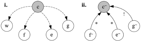
For the sake of concision, given ϵ=⟨aO, σ(aO)⟩∈Σ, for any o∈O,c∈C we refer to aO(o) as ϵ(o) and to σ(aO)(c) as ϵ(c). For illustration, consider an example from [Shih et al., 2018], in which a university admissions decision c is predicted using a BC with 4 observations: prior work experience, first-time applicant, passed entrance exam and met GPA. The graph in Figure 1i visualises, for this BC, O = {w, f, e, g}, C = {c}, and D = {(c, w), (c, f), (c, e), (c, g)}. This BC is binary, i.e. ∀x ∈ X , V(x) = {+, -}. The first column in Table 1 gives Σ for the BC in this example, amounting to 16 possible evaluations, with each row an evaluation in Σ (e.g. the first row amounts to ϵ with observations and classification all assigned to -, with e.g. ϵ(w) = - and ϵ(c) = -).
Our definition of BC does not include any probabilistic information, but the evaluations result from an underlying probability distribution, obtained when the classifier is learnt, but compiled away in providing evaluations (e.g. by setting the classifier to predict the most likely classification for a set of observations). For example, in the university admissions BC, σ amounts to a simple decision function, which may result from the use of a threshold t to determine a positive result for an assignment to observations if the probability of the single classification c being positive, given the assignments, is equal to or greater than t. The representation of BCs as sets of evaluations Σ/decision functions is a popular topic of late when explaining their output (e.g. see [Shih et al., 2019]). Indeed, some argue that explanations based on simple relational considerations are preferred to explanations resorting to more complex conceptual machineries (e.g. probabilistic considerations) [Lombrozo, 2007]. Note that the problem of extracting Σ is not the focus of this paper.
| Σ | CFX | MCX | PIX |
|---|---|---|---|
| w f e g | c R!(c)/R∗(c) | (¯w¯ f)(¯w¯ e)(¯w¯ g)(¯ f ¯ g)(¯ e¯ | |
| - - - - - - - - + | {}/{¯w ¯ f ¯ e¯ g} - {¯w}/{¯ f ¯ e} | (¯w¯ f)(¯w¯ e)(¯w¯ g)(¯ f ¯ g)(¯ e¯ g) (¯w ¯ f)(¯w¯ e) | g) (¯w ¯ f)(¯w¯ e) |
| - - + - - | {}/{¯w ¯ f ¯ g} | (¯w ¯ f)(¯w¯ g)(¯ f ¯ g) | (¯w ¯ f)(¯w¯ g)(¯ f ¯ g) |
| - - + + - | {¯w ¯ f}/{} | (¯w ¯ f) | (¯w ¯ f) |
| {}/{¯w¯ e¯ g} | (¯w¯ e)(¯w¯ g)(¯ e¯ g) | (¯w¯ e)(¯w¯ g)(¯ e¯ g) | |
| - + - - - | {¯w¯ e}/{} | (¯w¯ e) | (¯w¯ e) |
| - + - + - | {¯w¯ g}/{} | (¯w¯ g) | (¯w¯ g) |
| - + + - - | (f | ||
| - + + + + | {feg}/{} | (f eg) | eg) |
| + - - - - | {¯ g}/{¯ f ¯ e} | (¯ f ¯ g)(¯ e¯ g) | (¯ f ¯ g)(¯ e¯ g) (wg) |
| + - - + + | {wg}/{} {¯ | (wg) (¯ f ¯ g) | (¯ f ¯ g) |
| + - + - - | f ¯ g}/{} | (wg) | (wg) |
| + - + + + | {wg}/{e} | (¯ e¯ g) | (¯ e¯ g) |
| + + - - - | {¯ e¯ g}/{} | ||
| + + - + + | {wg}/{f} | (wg) | (wg) |
| + + + - + | {wfe}/{} | (wf e) | (wf e) |
| + + + + + | {}/{wfeg} | (wg) | (wg)(wf e)(f eg) |
In our definition of BCs, variables may have different domains or share the same domains. BCs can be binary, when the domains of variables consist of exactly two values, e.g. V(x) = {+, -} for all x ∈ X (as in the university admissions BC), or multidimensional (non-binary), where no restrictions are imposed on the domains of variables.
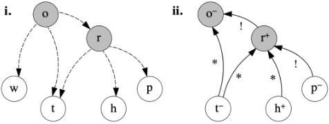
Finally, BCs may be single- or multi-label, depending on whether C is a singleton or not, respectively. Single-label BCs may be naive (as in the illustration for university admissions), when there are no conditional dependencies between observations. An example of a binary multi-label BC is shown graphically in Figure 2i. This BC determines the classifications play outside and raining based on the observations windy, temperature, humidity and pressure. We thus have C = {o, r}, O = {w, t, h, p}, D as in the figure, and Σ as in Table 2, where, e.g. when all the observations are (assigned to) + (bottom row), raining is (assigned to) - and play outside is (assigned to) +.
We will define counterfactual explanations in terms of the variables that may influence (assignments to) classifications:
Definition 2. The influences of a BC ⟨O, C,D, V, σ⟩ are I ⊆
| Σ | CFX | MCX | PIX | |
|---|---|---|---|---|
| w t h p r o | R!(r)/R∗(r) | R!(o)/R∗(o) | ||
| - - - - + - | {¯ t¯ p}/{} | {r}/{¯ t} | (¯ t)(¯ p) | (¯ t¯ p) |
| - - - + - + | {p}/{¯h} | { ¯w¯ r}/{} | (p) | (p) |
| - - + - + - | {¯ p}/{¯ th} | {r}/{¯ t} | (¯ t)(¯ p) | (h¯ p)(¯ t¯ p) |
| - - + + - + | {p}/{} | { ¯w¯ r}/{} | (p) | (p) |
| - + - - - + | {t¯h}/{} | {¯ r}/{ ¯wt} | (t) | (t¯h) |
| - + - + - + | {}/{t¯hp} | {¯ r}/{ ¯wt} | (t)(p) | (t¯h)(p) |
| - + + - + - | {h¯ p}/{} | {r}/{} | (¯ p) | (h¯ p) |
| - + + + - + | {p}/{t} | {¯ r}/{ ¯wt} | (t)(p) | (p) |
| + - - - + - | {¯ t¯ p}/{} | {}/{w¯ tr} | (¯ t)(¯ p) | (w¯ t)(¯ t¯ p) |
| + - - + - - | × | {w¯ t}/{} | (¯ t) | (w¯ t)(p) |
| + - + - + - | {¯ p}/{¯ th} | {}/{w¯ tr} | (¯ t)(¯ p) | (w¯ t)(h¯ p)(¯ t¯ p) |
| + - + + - - | × | {w¯ t}/{} | (¯ t) | (w¯ t)(p) |
| + + - - - + | {t¯h}/{} | {t¯ r}/{} | (t) | (t¯h) |
| + + - + - + | {}/{t¯hp} | {t¯ r}/{} | (t)(p) | (t¯h)(p) |
| + + + - + - | {h¯ p}/{} | {r}/{w} | (¯ p) | (h¯ p) |
| + + + + - + | {p}/{t} | {t¯ r}/{} | (t)(p) | (p) |
{(α, β) ∈ X × C∣β ∈ D(α)}. For any (α, β) ∈ I, we refer to α as the influencer and to β as the influencee; also, the influencers of α ∈ X are given by I(α) = {β ∈ X ∣(β, α) ∈ I}.
Intuitively, (α,β) should be in I if the value of influencer α may have an impact on the value of influencee β given by the BC. We choose binary, rather than more complex, influences to fulfil a desideratum of simplicity. We allow I to be any subset of X×C; the specific choice of I depends on the BC/classification task. In the university admissions BC, I ={(w,c),(f,c),(e,c),(g,c)}=O×C, thus each observation may influence the classification, while in the play-outside BC, I={(w,o),(t,o),(t,r),(h,r),(p,r),(r,o)}, thus classification r and observations w and t may all influence o. For more complex BCs, other forms of influences may be required, e.g. using Markov blankets [Pearl, 1989]. Note that naive BCs induce shallow graphs of influences, whereas multi-label BCs may induce non-shallow graphs.
Our counterfactual explanations are defined to answer the question "Why does the classification e ∈ C (the explanandum) have the value ϵ(e) in the context of the evaluation ϵ ∈ Σ?" They rely upon a selection of variables Xr ⊆ X, including the explanandum e, deemed to be relevant to e, as well as (two, mutually exclusive) relations between these variables, drawn from the restriction of the influences to the relevant variables and "chaining" (via "paths") the relevant variables Xr to e, where, as conventional, a path from A to B by a relation R is a sequence of distinct variables α1, . . . , αk, k ≥ 1, such that α1 = A, αk = B, and for each i, 1 ≤ i < k, (αi,αi+1) ∈ R. The motivation for Xr is that only some of the variables in X (potentially very few [Miller, 2019]) may suffice to explain the value assigned to e by ϵ. Formally:
Definition 3. Given a BC ⟨O, C, D, V, σ⟩ with influences I, a counterfactual explanation (CFX) for an explanandum e ∈ C in an evaluation ϵ ∈ Σ is a triple ⟨Xr,R!,R∗⟩ such that:
- R! ⊆ I is a binary relation of critical influence where ∀(α, β) ∈ R!, ∀γ ∈ I(β)/{α},
- ∃≥1ϵ′ ∈ Σ such that ϵ′ (γ) = ϵ(γ) and ϵ′ (α) ≠ ϵ(α) and
- ∀ϵ′ ∈Σ if ϵ′ (γ)=ϵ(γ) and ϵ′ (α)≠ϵ(α) then ϵ′ (β)≠ϵ(β); ● R∗ ⊆ I is a binary relation of potential influence where ∀(α, β) ∈ R∗:
- (α, β) ∉ R!;
- ∃ϵ′ , ϵ′′ ∈ Σ such that ϵ(α) = ϵ′ (α) ≠ ϵ′′ (α), ϵ(β) = ϵ′ (β) ≠ ϵ′′ (β) and ∀γ ∈ I(β)/{α}, ϵ′ (γ) = ϵ′′ (γ);
- {e} ⊆ Xr ⊆ X such that ∀α ∈ Xr/{e} there exists a path from α to e by R! ∪ R∗.
The critical influencers (CIs) and potential influencers (PIs) of any α ∈ X are defined as R!(α) = {β ∈ Xr∣(β,α) ∈ R!} and R∗(α) = {β ∈ Xr∣(β, α) ∈ R∗}, respectively.
The relations of critical and potential influence are based on the notion that if a change away from the current evaluation of an influencer may see a change in the evaluation of its influencee (when all its other influencers' evaluations remain unchanged), the influencee's current state somewhat depends on that of the influencer. A critical influence is a relation where any change in the evaluation of the influencer (with other influencers unchanged) will have this effect, thus it represents an immediate change which can be guaranteed. Meanwhile, a potential influence is not "critical" in that there exists at least one such possible change when other influencees remain in some constant (not necessarily the current) state, and thus it represents the possibility of such a change.
For illustration, the CFXs for the university admissions BC are shown in Table 1. Consider the evaluation with w ¯ f ¯ e¯ g, whose CFX, shown in Figure 1ii, includes a CI relation from ¯ g. If a change in the evaluation of g from - to + were seen with all other influencers remaining unchanged, the classification would also change from - to +. This CFX also shows that the relations from ¯ f and ¯ e are PIs, indicating the presence of some other case where a change in their evaluations from - to + would lead to a change in the classification from - to + (e.g. w ¯ f e¯ g to wfe¯ g for ¯ f and ¯wf¯ eg to ¯wfeg for ¯ e).
Note that CFXs can be understood as sub-graphs of the graph of influences, including (an assignment to) a classification (the explanandum) and with edges drawn from the two relations R! and R∗. If the given BC is naive, as for university admissions, then these sub-graphs (the CFXs) are shallow. Consider instead the multi-label play-outside BC, with CFXs for the classification o shown in Table 2. These CFXs now make use of other classifications and are thus non-shallow (e.g. the evaluation with ¯w¯ th¯ p admits the CFX in Figure 2ii, including the intermediate classification r explained in turn).
3 Formal Properties of CFXs
Here we prove that CFXs provide not only insights into the pivotal factors which lead to a classification but also potential changes which may result in different classifications. First we show uniqueness and (conditional) non-emptiness of CFXs.
Theorem 1. Given a BC ⟨O, C, D, V, σ⟩ and its influences I, let e ∈ C be an explanandum in an evaluation ϵ ∈ Σ. Then, ∃1⟨Xr,R!,R∗⟩ for e in ϵ, and if R! ∪R∗ = ∅ then ∄ϵ′ , ϵ′′ ∈ Σ such that ∃1α ∈ I(e) where ϵ′′ (α) ≠ ϵ′ (α) = ϵ(α), ϵ′′ (e) ≠ ϵ′ (e) = ϵ(e) and ∀β ∈ I(e)/{α}, ϵ′′ (β) = ϵ′ (β).
Proof. Follows fromDefinition 3.
We posit that the guarantee of a single, non-empty explanation is desirable, as it increases the chance of a user comprehending it and not being overwhelmed by multiple distinct explanations. We guarantee that the CFX (of an explanandum) is non-empty in the likely case that there are two distinct evaluations where changing the evaluation of a single influencer changes that of the influencee (the explanandum).
We now show CFXs are "compositional", in that they include CFXs of other classifications. Formally:
Theorem 2. Given a BC ⟨O, C,D,V,σ⟩, its influences I, and a CFX ⟨Xr,R!,R∗⟩ for an explanandum e ∈ C in an evaluation ϵ ∈ Σ, a CFX ⟨X ′ r ,R′! ,R′∗ ⟩ for any explanandum e′ ∈ C ∩Xr in ϵ is such that X ′ r ⊆ Xr, R′! ⊆ R! and R′∗ ⊆ R∗.
Proof. (Sketch) Whether in the context of ⟨Xr,R!,R∗⟩ or ⟨X ′ r ,R′! ,R′∗ ⟩, Definition 3 does not differ in determining R!(e′ ) or R′! (e′ ), R∗(e′ ) or R′∗ (e′ ) and, thus, the relevant variables linked by these relations Xr(e′ ) or X ′ r (e′ ), and thus their relations, and so on. Therefore, the theorem holds.
We thus simplify explanations of multi-label BCs since an explanation of a set of classifications may be represented by a single CFX. For example, for the play-outside BC, in all of the CFXs for o where r is present, the critical and potential influences towards r (and thus the relevant variables linked by these relations) are as in the corresponding CFX for r.
Our next result concerns the effect of changing the evaluation of an explanandum's CIs.
Theorem 3. Given a BC ⟨O, C,D,V,σ⟩, its influences I, and a CFX ⟨Xr,R!,R∗⟩ for e ∈ C in ϵ ∈ Σ, let α, β ∈ X be such that there is a unique path α1,. . . ,αk (k ≥ 1) from α to β by I. Then, ∀ϵ′ ∈ Σ such that ∀γ ∈ I(α1)∪. . .∪ I(αk)/{α1,. . . ,αk-1}, ϵ′ (γ)=ϵ(γ) and ϵ′ (α)≠ϵ(α), if there exists the same unique path by R!, then ϵ′ (β)≠ϵ(β).
Proof. (Sketch) By induction on the length k of the path: the property trivially holds if k = 1 and thus α = β; also, if the property holds for k - 1 (k > 1) then it holds for k, since ϵ(αk) is influenced exclusively by I(αk)=αk-1. Indeed ∀γ ∈ I(αk)/{αk-1}, ϵ′ (γ) = ϵ(γ) since there is no path from α1 to γ by I. Then, if we assume that ϵ′ (αk-1) ≠ ϵ(αk-1), by Definition 3, if (αk-1,αk) ∈ R!, then ϵ′ (αk) ≠ ϵ(αk).
Since a change in the evaluation of any CI will see a change in the evaluation of its influencee, which will in turn see a change in the evaluation of its (critical) influencee and so on, it becomes apparent that one single change sees a guaranteed chain reaction of changes along a path by the CIs. For example, in the play-outside BC, if we consider the CFX for ¯w¯ th¯ p in Figure 2ii, there is a single, critical path from ¯ p to ¯ o via r. This not only shows the important factors in the classifications but also that: if the pressure were high (positive), it would not be raining and play outside would be positive.
Our final result concerns changing the evaluation of an explanandum's PI when its evaluation does not change.
Theorem 4. Given a BC ⟨O, C, D, V, σ⟩, its influences I, and a CFX ⟨Xr,R!,R∗⟩ for e ∈ C in ϵ ∈ Σ such that R!(e) = ∅ and R∗(e) ≠ ∅, let α ∈ R∗(e). Then, ∀ϵ′ ∈ Σ such that ϵ′ (e) = ϵ(e), ϵ′ (α) ≠ ϵ(α) and ϵ′ (β) = ϵ(β) ∀β ∈ I(e)/{α}, given a CFX ⟨X ′ r ,R′! ,R′∗ ⟩ for e in ϵ′ , it must hold that ∣R′∗ (e)∣ ≤ ∣R∗(e)∣ and (trivially) ∣R′! (e)∣ ≥ ∣R!(e)∣.
Proof. (Sketch) We consider the states of e's incoming influences from ϵ = ⟨Xr,R!,R∗⟩ to ϵ′ = ⟨X ′ r ,R′! ,R′∗ ⟩. For (α, e), by Definition 3, α either loses its status as a PI if ϵ′ (e) = ϵ(e) is no longer potentially influenced by ϵ′ (α) ≠ ϵ(α), or it remains a PI, as it cannot become a CI in ϵ′ as this would require a change from ϵ(e) to ϵ′ (e). For {(γ, e) ∈ R∗∣γ ∈ X/{α}}, the only modified evaluation is ϵ′ (α), and thus, by Definition 3, these PIs either remain so or become CIs. For {(δ, e) ∈ I/R∗∣δ ∈ X}, any influence in R′! ∪R′∗ must have already been in R∗ by Definition 3. Thus the theorem holds.
When a change in the evaluation of a PI does not result in a change in the evaluation of its influencee, this theorem shows that it may no longer be a PI, while other PIs of the influencee may become CIs. Thus, PIs may highlight an iterative path towards CIs. This is an important finding demonstrating the power of CFXs as it shows how the two relations work in symphony to allow a user to assess the counterfactual factors of a BC's predictions. For example, in the BC in Table 1, CFXs may provide an admissions officer with reasons for why an applicant was accepted or not, in the form of factors which could have reversed that decision. Let us take the case ¯w ¯ f ¯ e¯ g where the applicant was rejected (-). In the corresponding CFX, none of the observations are CIs, i.e. a change in any observation would not change the classification for the applicant (Theorem 3). However, all observations are PIs, i.e. they may provide an iterative path towards a change by increasing the number of CIs (Theorem 4). If we change the evaluation of the PI ¯w (so now the applicant has prior work experience) we obtain w ¯ f ¯ e¯ g, whose CFX in Figure 1ii shows that the change generates the CI ¯ g. Thus, if the applicant were to meet the GPA, the classification would also change (Theorem 3). At this point the admissions officer can see that had the applicant had prior work experience and met the GPA, the classification would be reversed.
4 RelatedWork
In this section we discuss related work from the literature, making formal comparisons with our work. We do not review methods for explaining general Bayesian networks such as those aiming to obtain the most probable explanation [Pearl, 1989] as these approaches seek to determine approximations of the evaluations, which is outside the scope of this paper.
Two types of explanations for naive BCs are defined in [Shih et al., 2018]. We re-define them here so that they can be formally compared with our CFXs. The first form of explanation gives, for a positive (negative) classification, the minimal subset of the positive (negative, respectively) observations sufficient for the classification. The second form comprises the smallest set of variables that renders the other variables' evaluations irrelevant to the classification.
Definition 4. [Shih et al., 2018] Given a naive BC
⟨O, {c}, D, V, σ⟩ and an explanandum e = c in ϵ ∈ Σ: ● a minimum cardinality explanation (MCX) for e in ϵ is an evaluation m ∈ Σ such that m(e) = ϵ(e) and ∄ϵ′ ∈ Σ where ϵ′ (e)=ϵ(e) and ∣{o∈O∣ϵ′ (o)=ϵ(e)}∣<∣{o∈O∣m(o)=ϵ(e)}∣;
- a prime implicant explanation (PIX) for e in ϵ is a partial evaluation 2 p ∈ 2ϵ which is minimal (wrt set inclusion) and
- ∄ϵ′ ∈ Σ where ϵ′ ⊇ p and ϵ′ (e) ≠ ϵ(e).
Let M be the set of all MCXs and P be the set of all PIXs.
The formal relationship between PIXs and CFXs follows.
Theorem 5. Given a binary, naive BC ⟨O, {c},D,V,σ⟩, its influences I, and a CFX explanation ⟨Xr,R!,R∗⟩ for an explanandum e = c in ϵ ∈ Σ: ⋂p∈P p = R!(e).
Proof. For a variable x, let x ∈ ⋂p∈P p and suppose by contradiction x ∉ R!(e). This implies that ∃ϵ′ ∈ Σ such that ∀y ∈ X/{x}ϵ′ (y) = ϵ(y) while ϵ′ (x) ≠ ϵ(x). It follows that the partial evaluation p′ obtained restricting ϵ′ to X/{x} is either a PIX for e or there is a partial evaluation p′′ ⊊ p′ which is a PIX for e. Then there is a PIX for e not including x which contradicts the hypothesis x ∈ ⋂p∈P p. Conversely assume that x ∈ R!(e) but x ∉ ⋂p∈P p. Then ∃pj ∈ P such that x ∉ pj , and thus the partial evaluation pj can be extended to an evaluation ϵ′ such that ϵ′ (x) ≠ ϵ(x) while ∀y ∈ X/{x}ϵ′ (y) = ϵ(y) (in particular ϵ′ (e) = ϵ(e)) which contradicts x ∈ R!(e).
Since PIXs and MCXs are the most similar in the literature to our CFXs, we have provided illustrations thereof throughout the paper, and will use them as baselines in Section 5.
The explanations of [Timmer et al., 2015] also show the interplay between variables, utilising argumentation frameworks [Simari and Rahwan, 2009] as the reasoning model. A notion of support, similar to our influence, is used to derive evidential (rather than counterfactual) support graphs based on the Markov blanket of each variable (rather than only classifications in our method). Support graphs may contain multiple instances of a variable, whereas our CFXs do not.
Explanation trees for causal Bayesian networks [Nielsen et al., 2008] also use the variables relevant to explanations for explananda, but only for observations. The explanations are causal wrt the dataset, i.e. variable α causing variable β may affect the explanation, whereas ours are causal only wrt the BC itself, answering "what caused the BC to predict ϵ(e)?".
Various model-agnostic explanation methods exist, e.g. [Ribeiro et al., 2016; Lundberg and Lee, 2017], including some that generate counterfactuals, e.g. [Schwab and Karlen, 2019], but they generate flat explanations, ignoring factors between inputs and outputs that CFXs may use.
5 Experiments
We now evaluate CFXs empirically with various datasets and BCs. Our experiments indicate that CFXs (i) are of appropriate cardinality and length (compared with PIXs and MCXs from Section 4); (ii) highlight paths via PIs towards CIs; and (iii) give meaningful information about BCs' predictions. The algorithm we use to generate R! for an explanandum e ∈ C in ϵ ∈ Σ has time complexity O(µ ⋅ ∑x∈I(e) ∣V(x)∣), while that for R∗ has time complexity O(µ ⋅ ∏x∈I(e) ∣V(x)∣), where µ is the constant time required to compute a classification. For a binary, naive BC that can be compiled into an OBDD [Shih et al., 2018], to find a CI for e we generate the sub-graph induced by ϵ, checking for all x ∈ I(e) that there is an outgoing edge leading into the opposite sink to that of the classification. This has time complexity O(∣I(e)∣), where µ was removed as the result can be determined from the OBDD. To find a PI for e, for each x ∈ I(e), we search for paths to - and + classifications, keeping the subsequent variables constant. In the worst case, the whole OBDD may be searched.
2 Here, we treat any ϵ ∈ Σ as a set.
For the experiments we consider three settings: the Congressional Voting Records dataset 3 , the Parole Violation dataset 4 and the Child Bayesian network 5 . The Voting Records dataset consists of 435 voting records, amounting to 16 key votes by (Republican or Democrat) Congressmen in the USA. We understand votes as observations and party membership of Congressmen as classifications. We binarise the dataset such that votes are either yes or not yes. The Parole Violation dataset consists of 675 records, amounting to cases of prisoners who either violated parole or not, understood as classifications. Numeric features of the dataset were mapped into categorical ones using uniform length intervals, giving 8 categorical features for each prisoner, understood as observations. Child is a multi-label Bayesian network that describes the incidence of 6 possible diseases in a baby. We understand six clinical reports and age (the BN's leaves) as observations that generate 1080 possible evaluations with presence/absence of one of the diseases as the main classification and all other variables as intermediate classifications. We built a binary, naive BC with test set accuracy of 89.3% for Voting Records and a non-binary, naive BC with test set accuracy of 87.3% for Parole Violation. For Child, we applied inference rules from Bayes' theorem to obtain the classifications. In each BC, classifications' values in evaluations are set to those with the highest probability.
Table 3 shows our results concerning the explanations' cardinality and length. 6 All explanations here are non-empty, though CIs only appear in a subset of the results, which is expected as the more observations and values involved, the less likely it is that any change in a single variable will guarantee a different classification. While MCXs include every observation and are usually singular, many PIXs are generated for each evaluation, despite their more compact length, which may prevent easy comprehension by users in some settings. This point is accentuated in the datasets, particularly for the PIXs for the Voting Records, as shown in Table 3, where a single evaluation may generate hundreds of PIXs and only 4% have a single PIX. Our CFXs, meanwhile, are unique (per evaluation) and their length is between the two baselines. In the results for Child, the lengths of the (still numerous) PIXs decrease due to the intermediate classifications that they have no way of representing, whereas the CFXs capture them, with a notable increase in CIs. Overall, we posit that our CFXs performwell against the baselines in these experiments.
3 http://archive.ics.uci.edu/ml/index.php
4 https://www.icpsr.umich.edu/icpsrweb/NACJD/studies/26521
5 https://www.bnlearn.com/bnrepository/discrete-medium.html
6 Note that we consider MCXs for Voting Records only as the two others are non-binary and [Shih et al., 2018] define MCXs formally for binary BCs only; we consider PIXs for all BCs given that their definition directly extends to the non-binary case [Shih et al., 2018].
| Dataset (size, ∣X /{e}∣) | Exp. | Mean | Number of explanations of length: 51-75%76-100% | ||||
|---|---|---|---|---|---|---|---|
| length | 0% | 1-25% | 26-50% | ||||
| Voting Records (435, 16) | MCX PIX CFX CFX! | 100% 42% 76% 3% | 0 0 0 375 | 0 10627 0 41 | 0 108023 40 14 1132 | 0 16828 161 5 691 | 485 0 234 0 |
| Parole Violation | PIX | 50% 75% | 0 | 141 0 | 35 | 438 | 10 202 |
| (675, 8) | CFX! | 3% | 126 | 2 | 0 | 0 | |
| Child | PIX | 0 0 | 3264 | 84 | 0 | 0 | |
| CFX | 0 | ||||||
| 547 | 0 | ||||||
| (1080, 18) | CFX | 13% | 0 | 108 | 972 | ||
| CFX! | 86% 29% | 0 | 330 | 749 | 1 | 0 | |
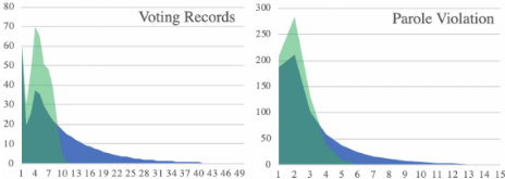
To show the usefulness of PIs in CFXs, we demonstrate that PIs can highlight paths towards CIs by performing path walk simulations. For the two naive BCs, for each evaluation we count the steps it takes to achieve a change in the classification. At each step, we select a CI to change if one is available, and if not, we select a PI and change it to the value which generates the lowest number of PIs in the modified evaluation's CFX. As a baseline, instead of selecting random PIs, we choose a random influencer. For the first case we also do not change any variable twice whenever possible, a strategy which causes dead ends in the baseline. Figure 3 shows the results when averaged over 1000 random seeds. We see much quicker convergence to a change with PIs, reducing the mean required steps from 9.5 to 4.7 and from 3.0 to 2.1 for Voting Records and Parole Violation, respectively.
Our final assessment pinpoints single CFXs to demonstrate their usefulness in real world situations. Consider an evaluation from the Voting Records BC where only water project cost sharing, physician fee freeze, El Salvador aid, religious groups in school, crime are positive, and this record is predicted to be from a Republican; a user may wish to know why this is the case. The CFX shows 13 PIs and 0 CIs, and changing one of these PIs, e.g. adoption of the budget resolution, does not change the prediction but means that the CFX now contains a CI, physician fee freeze (Theorem 4). Changing this CI changes the class to Democrat (Theorem 3) and the user is informed of two observations which were pivotal in the original classification. For this evaluation, 115 PIXs are generated (with a mean length of 8.0), a potentially overwhelming amount of information for a user, while the MCX gives physician fee freeze as its only (positive) variable. Clearly, other variables with a negative evaluation contributed towards this classification (in fact, changing this variable to - does not change the classification) but this information is lost in MCXs. This is due to the fact that they (by definition) do not discriminate between observations with a different evaluation to that of the classification. Another example can be seen in Table 2, where the observations windy and humidity are clearly factors in determining play outside (see the PIXs and CFXs), but they are not used by the MCXs as they affect it non-monotonically, e.g. when they are +, o is likely to be -.
In the context of the Parole Violation BC, we show the ability of CFXs to highlight problematic factors in classifications, e.g. to an expert user checking for bias. Consider the evaluation with observations female, white, 39-46y/o, other state, 5-6 prison, 11.8-13.4 sentence, multi-offender, larceny and classification non-violator. The CFX shows two CIs of white and female: a change in either one of these alone would change the classification, thus highlighting potential racial or sexist bias in the BC. Note that since Theorem 5 does not hold for non-binary BCs, this bias is not highlighted by PIXs.
Finally, in the Child BC, evaluation { LowerBodyO2=12+, LVHreport=no, XrayReport=Asy/Patchy, RUQO2=5-12, CO2Report=<7.5, GruntingReport=Yes, Age=0-3 days} has classification Disease=Lung, and the corresponding CFX shows a CI of LungParench=Abnormal, itself with a CI of Grunting=Yes. Each CI is a pivotal factor towards the evaluation (Theorem 2). Consideration of the intermediate classifications (i.e. BCs' internal reasoning) when explaining a classification is clearly useful in settings such as health but is absent in PIXs/MCXs, e.g. in Table 2, raining plays a huge role towards play outside and is included in all but two CFXs, but cannot be handled by PIXs and MCXs. Note that this would also be the case for the flat explanations generated by the model-agnostic methods mentioned in Section 4.
6 Conclusions
We have introduced a novel method for explaining the predictions of BCs via CFXs and have proven theoretically and provided some empirical evidence that the explanations are informative and appropriate for various settings. Our empirical results show for multiple datasets and BCs that CFXs provide important counterfactual information regarding the pivotal factors that could change a classification, opening up many applications for users ranging from non-experts (e.g counterfactually explaining a medical diagnosis) to experts (e.g. detecting bias in a BC in parole violation prediction).
For future work we will explore, from a HCI perspective, how CFXs should be delivered to users. We also plan to develop more efficient algorithms for the generation of R! and R∗. We will consider how other AI methods represented by decision functions could be explained by CFXs, e.g. (discretised) neural networks may be well suited to our method, with influences from inputs to intermediate features (e.g. see [Bau et al., 2017]) to outputs. Finally, we will compare with other (possibly probabilistic) notions for evaluating Bayesian networks, e.g. value of information measures [Chen et al., 2015] such as same-decision-probability [Choi et al., 2012].
@inproceedings{ijcai2020p63,
  title     = {Relation-Based Counterfactual Explanations for Bayesian Network Classifiers},
  author    = {Albini, Emanuele and Rago, Antonio and Baroni, Pietro and Toni, Francesca},
  booktitle = {Proceedings of the Twenty-Ninth International Joint Conference on
               Artificial Intelligence, {IJCAI-20}},
  publisher = {International Joint Conferences on Artificial Intelligence Organization},
  editor    = {Christian Bessiere},
  pages     = {451--457},
  year      = {2020},
  month     = {7},
  note      = {Main track},
  doi       = {10.24963/ijcai.2020/63},
  url       = {https://doi.org/10.24963/ijcai.2020/63},
}
TY - CPAPER TI - Relation-Based Counterfactual Explanations for Bayesian Network Classifiers AU - Albini, Emanuele AU - Rago, Antonio AU - Baroni, Pietro AU - Toni, Francesca T2 - Proceedings of the Twenty-Ninth International Joint Conference on Artificial Intelligence, IJCAI-20 PB - International Joint Conferences on Artificial Intelligence Organization PY - 2020 SP - 451 EP - 457 DO - 10.24963/ijcai.2020/63 UR - https://doi.org/10.24963/ijcai.2020/63 ER -Copied
Machine-readable versions of this paper, for tools and AI agents:





