
DACE: Distribution-Aware Counterfactual Explanation by Mixed-Integer Linear Optimization
Proceedings of the Twenty-Ninth International Joint Conference on Artificial Intelligence. Main track. Pages 2855-2862.
https://doi.org/10.24963/ijcai.2020/395
Keywords
- Machine Learning: Explainable Machine Learning
- Machine Learning: Classification
- Machine Learning: Interpretability
Abstract
Counterfactual Explanation (CE) is one of the post-hoc explanation methods that provides a perturbation vector so as to alter the prediction result obtained from a classifier. Users can directly interpret the perturbation as an "action" for obtaining their desired decision results. However, an action extracted by existing methods often becomes unrealistic for users because they do not adequately care about the characteristics corresponding to the empirical data distribution such as feature-correlations and outlier risk. To suggest an executable action for users, we propose a new framework of CE for extracting an action by evaluating its reality on the empirical data distribution. The key idea of our proposed method is to define a new cost function based on the Mahalanobis' distance and the local outlier factor. Then, we propose a mixed-integer linear optimization approach to extracting an optimal action by minimizing our cost function. By experiments on real datasets, we confirm the effectiveness of our method in comparison with existing methods for CE.
- [Ballet et al., 2019] Vincent Ballet, Xavier Renard, Jonathan Aigrain, Thibault Laugel, Pascal Frossard, and Marcin De- tyniecki. Imperceptible adversarial attacks on tabular data. In NeurIPS 2019 Workshop on Robust AI in Financial Ser- vices: Data, Fairness, Explainability, Trustworthiness and Privacy, 2019.
- [Breiman, 2001] Leo Breiman. Random forests. Machine Learning, 45(1):5-32, 2001.
- [Breunig et al., 2000] Markus M. Breunig, Hans-Peter Kriegel, Raymond T. Ng, and Jörg Sander. LOF: Iden- tifying density-based local outliers. SIGMOD Rec., 29(2):93-104, 2000.
- [Chen and Guestrin, 2016] Tianqi Chen and Carlos Guestrin. XGBoost: A scalable tree boosting system. In Proceedings of the 22nd ACM SIGKDD International Conference on Knowledge Discovery and Data Mining, page 785-794, 2016.
- [Cui et al., 2015] Zhicheng Cui, Wenlin Chen, Yujie He, and Yixin Chen. Optimal action extraction for random forests and boosted trees. In Proceedings of the 21th ACM SIGKDD International Conference on Knowledge Discov- ery and Data Mining, page 179-188, 2015.
- [Dhurandhar et al., 2018] Amit Dhurandhar, Pin-Yu Chen, Ronny Luss, Chun-Chen Tu, Paishun Ting, Karthikeyan Shanmugam, and Payel Das. Explanations based on the missing: Towards contrastive explanations with pertinent negatives. In Proceedings of the 32nd International Con- ference on Neural Information Processing Systems, page 590-601, 2018.
- [Dua and Graff, 2017] Dheeru Dua and Casey Graff. UCI machine learning repository, 2017.
- [FICO et al., 2018] FICO, Google, Imperial College Lon- don, MIT, University of Oxford, UC Irvine, and UC Berkeley. Explainable Machine Learning Challenge, 2018.
- [Friedman, 2000] Jerome H. Friedman. Greedy function ap- proximation: A gradient boosting machine. Annals of Statistics, 29:1189-1232, 2000.
- [Ghorbani et al., 2019] Amirata Ghorbani, Abubakar Abid, and James Y. Zou. Interpretation of neural networks is fragile. In Proceedings of the Thirty-Third AAAI Confer- ence on Artificial Intelligence, pages 3681-3688, 2019.
- [Guidotti et al., 2018] Riccardo Guidotti, Anna Monreale, Salvatore Ruggieri, Franco Turini, Fosca Giannotti, and Dino Pedreschi. A survey of methods for explaining black box models. ACM Comput. Surv., 51(5), 2018.
- [Hastie et al., 2009] Trevor Hastie, Robert Tibshirani, and Jerome H. Friedman. The Elements of Statistical Learn- ing: Data Mining, Inference, and Prediction, 2nd Edition. Springer Series in Statistics. Springer, 2009.
- [IBM, 2018] IBM. CPLEX Optimizer -IBM. https://www. ibm.com/analytics/cplex-optimizer, 2018. Link
- [Ke et al., 2017] Guolin Ke, Qi Meng, Thomas Finley, Taifeng Wang, Wei Chen, Weidong Ma, Qiwei Ye, and Tie-Yan Liu. LightGBM: A highly efficient gradient boosting decision tree. In Proceedings of the 31st Interna- tional Conference on Neural Information Processing Sys- tems, page 3149-3157, 2017.
- [Koh and Liang, 2017] Pang Wei Koh and Percy Liang. Un- derstanding black-box predictions via influence functions. In Proceedings of the 34th International Conference on Machine Learning -Volume 70, page 1885-1894, 2017.
- [Kulis, 2013] Brian Kulis. Metric learning: A survey. Foun- dations and Trends in Machine Learning, 5(4):287-364, 2013.
- [Lash et al., 2017] Michael T. Lash, Qihang Lin, W. Nick Street, Jennifer G. Robinson, and Jeffrey W. Ohlmann. Generalized inverse classification. In Proceedings of the 2017 SIAM International Conference on Data Mining, pages 162-170, 2017.
- [Laugel et al., 2019a] Thibault Laugel, Marie-Jeanne Lesot, Christophe Marsala, and Marcin Detyniecki. Issues with post-hoc counterfactual explanations: a discussion. In 2019 ICML Workshop on Human in the Loop Learning, 2019.
- [Laugel et al., 2019b] Thibault Laugel, Marie-Jeanne Lesot, Christophe Marsala, Xavier Renard, and Marcin De- tyniecki. The dangers of post-hoc interpretability: Unjus- tified counterfactual explanations. In Proceedings of the Twenty-Eighth International Joint Conference on Artificial Intelligence, pages 2801-2807, 2019. IJCAI
- [Lundberg and Lee, 2017] Scott M Lundberg and Su-In Lee. A unified approach to interpreting model predictions. In Proceedings of the 31st International Conference on Neu- ral Information Processing Systems, pages 4765-4774, 2017.
- [Maesschalck et al., 2000] R. De Maesschalck, D. Jouan- Rimbaud, and D.L. Massart. The mahalanobis dis- tance. Chemometrics and Intelligent Laboratory Systems, 50(1):1 -18, 2000.
- [Mahalanobis, 1936] Prasanta Chandra Mahalanobis. On the generalized distance in statistics. Proceedings of the Na- tional Institute of Sciences, 2:49-55, 1936.
- [Molnar, 2019] Christoph Molnar. Interpretable Machine Learning -A Guide for Making Black Box Models Explain- able. https://christophm.github.io/interpretable-ml-book/, 2019. Link
- [Moore et al., 2019] Jonathan Moore, Nils Hammerla, and Chris Watkins. Explaining deep learning models with con- strained adversarial examples. In Proceedings of the 16th Pacific Rim International Conference on Artificial Intelli- gence, pages 43-56, 2019.
- [Ribeiro et al., 2016] Marco Túlio Ribeiro, Sameer Singh, and Carlos Guestrin. "Why Should I Trust You?": Ex- plaining the predictions of any classifier. In Proceedings of the 22nd ACM SIGKDD International Conference on Knowledge Discovery and Data Mining, page 1135-1144, 2016.
- [Ribeiro et al., 2018] Marco Túlio Ribeiro, Sameer Singh, and Carlos Guestrin. Anchors: High-precision model- agnostic explanations. In Proceedings of the Thirty- Second AAAI Conference on Artificial Intelligence, pages 1527-1535, 2018.
- [Rudin, 2019] Cynthia Rudin. Stop explaining black box machine learning models for high stakes decisions and use interpretable models instead. Nature Machine Intelligence, 1:206-215, 2019.
- [Russell, 2019] Chris Russell. Efficient search for diverse coherent explanations. In Proceedings of the Confer- ence on Fairness, Accountability, and Transparency, page 20-28, 2019.
- [Szegedy et al., 2014] Christian Szegedy, Wojciech Zaremba, Ilya Sutskever, Joan Bruna, Dumitru Er- han, Ian J. Goodfellow, and Rob Fergus. Intriguing properties of neural networks. In Proceedings of the 2nd International Conference on Learning Representations, 2014.
- [Ustun et al., 2019] Berk Ustun, Alexander Spangher, and Yang Liu. Actionable recourse in linear classification. In Proceedings of the Conference on Fairness, Accountabil- ity, and Transparency, page 10-19, 2019.
- [Wachter et al., 2018] Sandra Wachter, Brent Mittelstadt, and Chris Russell. Counterfactual explanations without opening the black box: Automated decisions and the gdpr. Harvard journal of law & technology, 31:841-887, 2018.
References were extracted automatically from the PDF and may contain errors.
Full text extracted automatically from the PDF; figures, tables and equations may differ. The PDF is the version of record.
1 Introduction
1.1 Background andMotivation
In recent years, complex machine learning models, such as deep neural networks and tree ensemble models, have achieved high prediction accuracy and been widely used for assisting the decision-making tasks in the real world, such as medical diagnosis and loan approval. As a result, to understand not only why an undesired prediction is obtained, but also how to act to obtain a desirable outcome, post-hoc methods for extracting explanations from the individual prediction of complex models have increasingly been attracting attention [Guidotti et al., 2018; Molnar, 2019]. One of the post-hoc explanation approaches is the Counterfactual Explanation (CE) [Wachter et al., 2018]. For a given classifier H : X → Y, target class t ∈ Y, and instance ¯x ∈ X such that H(¯x) ̸= t, the aim of CE is to find an optimal solution a⋆ of the following optimization problem:
where A is a set of actions, and C : A → R≥0 is a cost function that measures the required efforts of an action a ∈ A. This problem is related to the adversarial examples [Szegedy et al., 2014] in the sense that it finds a perturbation a that alters the output of a classifier H. In the context of CE, on the other hand, an action a is interpreted as a required action for a user ¯x to obtain the desired prediction result (e.g., low risk of default). Therefore, the action suggested by CE should be executable for users. In this paper, we focus on this characteristic property of CE, and discuss how to provide a realistic action so that users can directly refer to and execute.
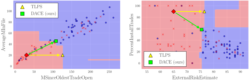
To extract realistic actions, we need to define a cost function C that considers the empirical distribution. While several useful cost functions, such as the total log-percentile shift (TLPS) [Ustun et al., 2019], have been proposed, we argue that they often extract unrealistic actions. Figure 1 presents two demonstrations on the FICO dataset [FICO et al., 2018], which is a real dataset of Home Equity Line of Credit (HELOC) applications. The task is to predict whether individuals will default on their HELOC. Figure 1 shows actions a (yellow arrows) extracted by using the TLPS from random forest classifiers trained on the dataset, and these modified instances ¯x + a (yellow triangles). Table 1(a) shows the actual values of them. From Figure 1, we can observe that these modified instances ¯x + a are located in the region predicted as "low risk of default", however, we argue that these actions are not realistic for users from the following two perspectives corresponding to the characteristics of the empirical distribution:
- Feature-correlation: Because each feature is often dependent on others, having non-zero correlation, the cost of changing a value with respect to a feature should be evaluated depending both on the amount of its difference and relation to other features. In Figure 1 (left), it seems unnatural to increase only "MSinceOldestTradeOpen" without increasing "AverageMInFile" because these features are correlated.
- Outlier risk: By minimizing the cost of a, there is a risk that its modified instance ¯x + a becomes an outlier of the empirical distribution. In Figure 1 (right), it seems unrealistic to increase "ExternalRiskEstimate" without decreasing "PercentInstallTrades", because there are no training instances near ¯x + a.
Based on the above observations, our goals are (i) to model
| Feature to Change | Action | MD | LOF |
|---|---|---|---|
| "MSinceOldestTradeOpen" | 30→126 (+96) | 4.39 | 1.93 |
| "ExternalRiskEstimate" | 65→77 (+12) | 1.35 | 7.92 |
(a) TLPS [Ustun et al., 2019]
| Feature to Change | Action | MD | LOF |
|---|---|---|---|
| "MSinceOldestTradeOpen" "AverageMInFile" | 30→109 (+79) 20 → 46 (+26) | 1.11 | 1.17 |
| "ExternalRiskEstimate" "PercentInstallTrades" | 65→76 (+11) 90 → 58 (-32) | 1.40 | 1.04 |
(b) DACE (ours)
Table 1: Examples of CE extracted on the FICO dataset. These actions provide how to change feature values so as to be predicted as "low risk of default" from the classifier learned on the dataset.
the reality of an action as a cost function C, and (ii) to propose a method to optimize C for extracting realistic actions.
1.2 Our Contributions
In this paper, we propose a new framework of CE, named Distribution-Aware Counterfactual Explanation (DACE), that extracts a realistic action for users. Our contributions can be summarized as follows:
- We propose a new cost function based on the Mahalanobis' distance (MD) [Mahalanobis, 1936] and Local Outlier Factor (LOF) [Breunig et al., 2000] to evaluate the reality of actions. MD is known as a metric that captures the relationships between features, and LOF is a popular outlier score that measures how unusual a given instance is by using k-nearest neighbor (k-NN).
- We formulate the problem of finding an optimal action according to our cost function as a mixed-integer linear optimization (MILO) problem, which can be solved by modern MILO solvers, such as CPLEX [IBM, 2018].
For computational efficiency, we show that if we use ℓ1-norm based MD and 1-NN based LOF for the cost function, the number of variables and constraints of the problem can be reduced dramatically.
- We demonstrate the effectiveness of DACE compared to other existing methods including MAD [Wachter et al., 2018; Russell, 2019], TLPS [Ustun et al., 2019], and PCC [Ballet et al., 2019] on real datasets.
Table 1(b) and the green arrows in Figure 1 show the actions extracted by our DACE. These results suggest that the MD and LOF of actions reflect the feature-correlations and outlier risks well, respectively, and that DACE can extract realistic actions in the sense of these properties.
1.3 RelatedWork
Counterfactual Explanation. Anumber of post-hocmethods for generating explanations from complex models have been proposed [Ribeiro et al., 2016; Lundberg and Lee, 2017; Koh and Liang, 2017; Ribeiro et al., 2018]. Counterfactual Explanation (CE) is one of the post-hoc methods that has been attracting attention in recent years. Most of existing CE methods are either gradient-based [Wachter et al., 2018; Dhurandhar et al., 2018; Moore et al., 2019] or heuristic search [Lash et al., 2017]. These methods can deal with differentiable models over continuous features. On the other hand, there have been increasing demands for learning non-differentiable models over possibly non-continuous features such as tree ensembles over categorical data, to which existing gradient-based methods are not applicable. To overcome these difficulties, several authors proposed integer linear optimization (ILO) approaches [Cui et al., 2015; Ustun et al., 2019; Russell, 2019], using linear costs. Our results extend their approach to a cost function containing nonlinear terms such as MD and LOF.
Distribution-aware score for CE. Recently, some studies have pointed out the risk that existing post-hoc methods often suffer from a lack of robustness [Ghorbani et al., 2019; Rudin, 2019]. For this problem, the following scores for CE
were proposed. [Laugel et al., 2019b] has introduced the notion of connectedness of an action to exclude a meaningless action that transfers a given data to an empty decision region containing no training data. They also pointed out that most of existing CE methods can generate non-connected actions. Note however that their connectedness and our criterion are incomparable. Actually, in Figure 1, all the actions are connected, while some of them are classified as bad according to our criterion. Another distribution-aware criterion, called proximity [Laugel et al., 2019a] for CE, is related to the LOF. To the best of our knowledge, our method is a first attempt to optimize it, while the above work proposed criteria only.
2 Preliminaries
2.1 Notations and Settings
For a positive integer n ∈ N, we denote by [n] := {1, . . . , n}. For a proposition ψ, I [ψ] denotes the indicator of ψ, i.e., I [ψ] = 1 if ψ is true, and I [ψ] = 0 if ψ is false.
Throughout this research, we consider a binary classification problem as a prediction task, which is sufficient for CE. For a multi-class classification problem, we can reduce it to a binary classification problem between the target class and other classes. We denote input and output domains by X = X1 × · · · ×XD ⊆ RD and Y = {-1, +1}, respectively. Let a vector x = (x1, . . . , xD) ∈ X be an instance, and a function H : X → Y be a classifier.
We assume that categorical features included by a dataset are one-hot encoded by pre-processing. Let G ⊆ [D] be a set of features that represents a one-hot encoded categorical feature with |G| categories. Then, Xg = {0, 1} for g ∈ G and ∑g∈G xg = 1 for any x ∈ X . We denote a set of one-hot encoded categorical features G by G ⊆ 2[D] .
2.2 Mahalanobis' Distance (MD)
The Mahalanobis' distance (MD) is a popular metric in the literature on statistics and metric learning [Mahalanobis, 1936; Kulis, 2013]. For two vectors x, x′ ∈ RD and a positive semi-definite matrix M ∈ RD×D , Mahalanobis' distance dM : RD × RD → R≥0 between x and x′ is defined by
Since M is positive semi-definite, M can be decomposed as M = U ⊤U, where U ∈ RD×D . Hence, dM(x, x′ | M) can be also expressed as follows:
where ‖ · ‖p denotes the ℓp-norm. In statistics, the inverse matrix of the covariance matrix Σ of the distribution where x and x′ follow is often used as M. It is known that the MD d(x, x′ | Σ-1 ) is scale-invariant and takes the feature correlations into account [Maesschalck et al., 2000].
2.3 Local Outlier Factor (LOF)
The local outlier factor (LOF) is a prominent outlier score based on the local densities of instances [Breunig et al., 2000]. We assume a metric space (X,∆) and a set of N instances X ⊆ X . We omit them if it is clear from context. For x ∈ X, let Nk(x) be its k-nearest neighbors (k-NN) on X. The k-reachability distance rdk of x with respect to x′ is defined by rdk(x, x′ ) := max{∆(x, x′ ), dk(x′ )}, where dk(x′ ) is the distance ∆ between x′ and its the k-th nearest instance on X. The k-local reachability density of x is defined by lrdk(x) := |Nk(x)| · (∑x′∈Nk(x) rdk(x, x′ ))-1 . Then, the k-LOF of x on X is defined as follows:
As a metric ∆ : X × X → R≥0, we assume ∆(x, x′ ) = ∑Dd=1 ∆d(xd, x′ d), where ∆d : Xd × Xd → R≥0 is some dissimilarity measure of the feature d ∈ [D].
2.4 Additive Classifiers
In this paper, we focus on additive classifiers H : X → Y expressed as the following additive form:
where h1, . . . , hT : X → R are base learners, wt ∈ R is a weight value of ht for t ∈ [T ], and b ∈ R is an intercept.
Linear Model. Linear models (LM), such as Logistic Regression and Linear Support Vector Machines, are one of the most standard classifiers [Hastie et al., 2009]. If H is a LM, T = D and each base learner hd(x) = xd. A LM makes a prediction depending on the sign of the inter product 〈w, x〉, where w = (w1, . . . , wD) ∈ RD .
Tree EnsembleModel. Tree ensemble models (TEM), such as Random Forest [Breiman, 2001] and Gradient Boosted Trees [Friedman, 2000; Chen and Guestrin, 2016; Ke et al., 2017], are renowned for their high prediction performances in machine learning competitions. If H is a TEM, each base learner ht is a decision tree, which is a classifier that consists of a set of if-then-else rules expressed by a binary tree structure. It makes the prediction according to a leaf that the input instance x ∈ X reaches, and the corresponding leaf is determined by traversing the tree from the root depending on whether the statement xd ≤ t is true or not, where d ∈ [D] and t ∈ R are a pair of parameters corresponding to the internal node. A TEM makes a prediction by combining the prediction results from T decision trees.
3 Problem Statement
3.1 Action and Action Set
For a classifier H : X → Y, and an instance ¯x ∈ X such that H(¯x) = -1, we define an action as a perturbation vector a ∈ RD such that H(¯x + a) = +1. An action set A = A1 × · · · × AD is a finite set of feasible actions such that 0 ∈ Ad and Ad ⊆ {a ∈ R | ¯xd + ad ∈ Xd} for d ∈ [D]. We denote by Id = |Ad| for d ∈ [D].
We can automatically determine each Ad depending on the type of the classifier H [Ustun et al., 2019; Cui et al., 2015] and the feature d ∈ [D]. For example, if xd is a feature representing "age", then ad ∈ N∪{0} holds for any ad ∈ Ad. If xd is an immutable feature (e.g., gender) then Ad = {0}.
3.2 Cost Function
As a score to evaluate whether an action is realistic for users, we introduce a new cost function CDACE : A → R≥0. Given a positive semi definite matrix M ∈ RD×D , set of N instances X ⊆ X, positive integer k ∈ [N], and λ ≥ 0, we define CDACE with respect to an input instance ¯x ∈ X as
where
- d2M(¯x, ¯x + a | M) is the squared MD between the input instance ¯x and its modified instance ¯x + a,
- qk(¯x+a | X) is the k-LOF of ¯x+a on X, and
- λ ≥ 0 is a trade-off parameter between d2M and qk.
3.3 ProblemDefinition
Our aim is to find an action a ∈ A that minimizes the cost CDACE(a | ¯x), and this problem can be defined as follows:
Problem 1. Given an additive classifier H : X → Y, input instance ¯x ∈ X such that H(¯x) = -1, positive semi definite matrix M ∈ RD×D , set of N instances X ⊆ X , positive integer k ∈ [N], and λ ≥ 0, find an action a∗ ∈ A such that is an optimal solution for the following optimization problem:
4 MILO Formulation
In this section, we propose an MILO formulation for solving Problem 1.
4.1 Basic Ideas
While CDACE is non-linear and has a discrete structure caused by Nk(¯x + a), we can exactly formulate Problem 1 as an MILO problem using modeling techniques on integer optimization. However, to linearize the non-linearity and discreteness, this naive formulation requires O(|A|2 +N 2 ) auxiliary variables and constraints, where |A| := ∑Dd=1 |Ad|. Preliminary experiments made clear that this formulation was computationally infeasible on standard datasets.
In order to avoid introducing O(|A|2 + N 2 ) auxiliary variables and constraints, we introduce a surrogate objective function and optimize it instead of CDACE. Our main ideas are (i) fixing k = 1 for the LOF qk(¯x+a) of CDACE, and (ii) replacing the MD d2M of CDACE with ℓ1-norm based Mahalanobis' distance (ℓ1-MD) ˆ dM defined as
which is based on the fact that d2M can be expressed as dM(x, x′ | M) := ‖U(x′ - x)‖2. Overall, we formulate the following problem as an MILO problem instead of Problem 1:
First, we introduce binary variables πd,i ∈ {0, 1} for d ∈ [D] and i ∈ [Id], which indicate that the action ad,i ∈ Ad is selected (πd,i = 1) or not (πd,i = 0). Then, πd,i must satisfy the following constraints:
Each element of the action a = (a1, . . . , aD) ∈ A can be expressed as ad = ∑Id i=1 ad,iπd,i. Constraint (2) is corresponding to one-hot encoded categorical features G. In the rest of this section, we formulate the constraint and objective function by using linear constraints of πd,i.
4.2 Base Learner Constraints
Because the output value of each base learner ht for ¯x + a varies depending on the value of a, i.e., the program variables πd,i, we must express the value of ht(¯x + a) by linear constraints of πd,i. We introduce variables ξt ∈ R such that ξt = ht(¯x + a) for t ∈ [T]. From the definition of additive classifiers, the constraint H(¯x+a) = +1 is equivalent to the following linear constraint of ξt:
In the following, we show how to express ξt when H is a linear model (LM) or tree ensemble model (TEM).
Linear Models. From the definition of LM, T = D and hd(¯x + a) = ¯xd + ad holds for d ∈ [D]. Hence, we can simply express the base learner of the LM as follows:
Tree Ensemble Models. Each base learner ht of the TEM is a decision tree. It is known that a decision tree ht : X → Y with Lt leaves represents a partition {rt,1, . . . , rt,Lt } of the input domain X [Hastie et al., 2009], and can be expressed as ht(x) = ∑Ll=1 ˆ yt,l · I [x ∈ rt,l], where ˆ ym,l ∈ Y is a predictive label corresponding to the leaf l ∈ [Lt] of ht. In order to express the statement ¯x+a ∈ rt,l, we can utilize the decision logic constraint proposed by [Cui et al., 2015] expressed as
where I (d) t,l = {i ∈ [Id] | ¯xd + ad,i ∈ r(d) t,l } and r(d) t,l is the subspace of Xd such that rt,l = r(1) t,l × · · · × r(D) t,l . φt,l is an indicator variable such that φt,l = I [¯x + a ∈ rt,l]. Then, we can express the base learner of the TEM as follows:
Because I (d) t,l , Lt, and ˆ yt,l can be computed when H and A are given, they are constant values.
4.3 Surrogate Objective Function
ℓ1-norm based Mahalanobis' Distance (ℓ1-MD). The ℓ1MD between ¯x and ¯x + a can be expressed as follows:
where Ud = (Ud,1, . . . ,Ud,D) is the d-th row vector of U. We introduce variables δd ≥ 0 for d ∈ [D] such that δd = |〈Ud, a〉|. Then, ˆ dM(¯x, ¯x + a | M) can be expressed as
with the following constraints:
ˆ dM is not exactly the same as d2M however, we show the approximation ratio of ˆ dM with respect to d2M as follows:
Proposition 1. Let a∗ , ˆa ∈ RD be two vectors such that a∗ = arg mina∈RD d2M(¯x, ¯x + a | M) and ˆa = arg mina∈RD ˆ dM(¯x, ¯x + a | M), respectively. Then dM(¯x, ¯x + ˆa | M) ≤ √D · dM(¯x, ¯x + a∗ | M) holds.
Proof. Let U ∈ RD×D be a matrix such that M = U ⊤U. By the definitions, dM(¯x, ¯x + a | M) and ˆ dM(¯x, ¯x+ a | M) are expressed as dM(¯x, ¯x + a | M) = ‖Ua‖2 and ˆ dM(¯x, ¯x+ a | M) = ‖Ua‖1, respectively. From the properties of Lp-norm, it holds that ‖Uˆa‖2 ≤ ‖Uˆa‖1 and ‖Ua∗ ‖1 ≤ √D · ‖Ua∗ ‖2. Recall the definitions of a∗ and ˆa, ‖Uˆa‖1 ≤ ‖Ua∗ ‖1 holds. By combining these inequalities, we have ‖Uˆa‖2 ≤ √D · ‖Ua∗ ‖2, which is equivalent to dM(¯x, ¯x + ˆa | M) ≤ √D · dM(¯x, ¯x+a∗ | M). □
1-Local Outlier Factor (1-LOF). From the definitions of qk and lrdk, qk(¯x + a | X) for k = 1 can be expressed as
where m = arg minn∈[N] ∆(¯x + a, x(n) ), i.e., N1(¯x + a) = {x(m) }. Because m and rd1(¯x + a, x(m) ) varies depending on ¯x + a, i.e., the variables πd,i, we need to formulate it by linear constraints of πd,i. We introduce variables νn ∈ {0, 1} and ρn ≥ 0 for n ∈ [N] such that νn = I [x(n) ∈ N1(¯x + a)]
| #Vars | #Consts | #Vars | #Const | |
|---|---|---|---|---|
| d2M | O(|A|2 ) O(N 2 ) | O(|A|2 ) | ˆ dM O(D) | O(D) |
| Nk | O(N 2 ) | N1 O(N) | O(N 2 ) | |
| qk | O(N 2 ) | O(N 2 ) | q1 O(N) | O(N) |
and ρn = rd1(¯x+a, x(n) ) · νn, respectively. Then, q1(¯x+a) can be expressed as a linear form of ρn as follows:
with the following constraints:
where c(n) d,i , Cn, dn, and l(n) are constant values such that c(n) d,i = ∆d(¯xd + ad,i, x(n) d ), Cn ≥ maxa∈A∆(¯x + a, x(n) ), d(n) = d1(x(n) ), and l(n) = lrd1(x(n) ). Constraints (10) and (11) are based on the statement νm = 1 ⇒ ∀n ∈ [N] : ∆(¯x + a, x(m) ) ≤ ∆(¯x + a, x(n) ), which is for expressing the nearest instance of ¯x + a. Note that ∆(¯x + a, x(n) ) = ∑Dd=1 ∑Id i=1 c(n) d,i πd,i, and Constraints (12) and (13) are based on the definition of k-reachability distance rdk. All constant values can be computed when X and A are given.
4.4 Overall Formulation
Finally, we show our overall formulation as follows:
| Logistic Regression | Random Forest | |||||
|---|---|---|---|---|---|---|
| dM(¯x, ¯x+a | Σ-1 ) | q10(¯x+a | X+) | Time[s] | dM(¯x, ¯x+a | Σ-1 ) | q10(¯x+a | X+) | Time[s] | |
| MAD | 5.42 ± 4.04 | 1.65 ± 1.29 | 0.0261 ± 0.00439 | 2.29 ± 1.58 | 1.56 ± 1.14 | 34.4 ± 57.8 |
| TLPS | 9.09 ± 2.97 | 3.86 ± 1.49 | 0.0208 ± 0.00761 | 2.22 ± 1.31 | 1.49 ± 1.07 | 22.5 ± 36.6 |
| PCC | 9.46 ± 6.66 | 1.61 ± 1.31 | 0.0238 ± 0.0036 | 3.76 ± 2.36 | 1.6 ± 1.27 | 29.8 ± 78.7 |
| DACE | 1.97 ± 1.46 | 1.54 ± 1.12 | 67.9 ± 75.8 | 1.54 ± 1.18 | 1.33 ± 0.496 | 519 ± 171 |
| Logistic Regression | Random Forest | |||||
|---|---|---|---|---|---|---|
| dM(¯x, ¯x+a | Σ-1 ) | q10(¯x+a | X+) | Time[s] | dM(¯x, ¯x+a | Σ-1 ) | q10(¯x+a | X+) | Time[s] | |
| MAD | 8.89 ± 2.73 | 1.94 ± 3.41 | 0.0488 ± 0.00215 | 7.5 ± 6.12 | 1.91 ± 2.19 | 33.6 ± 47.1 |
| TLPS | 3.73 ± 2.26 | 1.78 ± 0.718 | 0.0113 ± 0.00163 | 2.44 ± 3.91 | 1.34 ± 0.75 | 133 ± 193 |
| PCC | 8.14 ± 3.15 | 1.94 ± 3.41 | 0.042 ± 0.0022 | 6.73 ± 4.12 | 1.95 ± 2.18 | 11.9 ± 10.9 |
| DACE | 2.27 ± 1.51 | 1.27 ± 0.35 | 1.03 ± 0.276 | 1.23 ± 1.34 | 1.13 ± 0.27 | 240 ± 239 |
Table 3: Experimental results on the FICO and german datasets.
Table 2 presents the numbers of variables and constraints required for the naive formulation of Problem 1 and the problem (14). It shows that the latter reduces variables and constraints dramatically compared to the former. Therefore, our DACE solves the problem (14) to extract the desired action for computational efficiency.
As with the existing ILO-based methods [Ustun et al., 2019; Russell, 2019], our formulation can be (i) efficiently solved by powerful off-the-shelf MILO solvers, such as CPLEX [IBM, 2018], (ii) customized by adding constraints that users desire, such as a limitation of features changed by actions, and (iii) applied to an algorithm for enumerating distinct actions as its subroutine. To summarize the above advantages, we can obtain actions that satisfy user-defined constraints without implementing designated algorithms.
5 Experiments
We conduct experiments on real datasets to investigate the effectiveness of our DACE by comparing the performance with existing methods for CE. All codes were implemented in Python 3.6 with scikit-learn and IBM ILOG CPLEX v12.8. All experiments were conducted on 64-bit Ubuntu 18.04.1 LTS with Intel Xeon E5-1620 v4 3.50GHz CPU and 62.8GiB memory, and we imposed a 600 second time limit for solving.
5.1 Experimental Setting
We used the FICO dataset (D = 23) [FICO et al., 2018] and german dataset (D = 61) [Dua and Graff, 2017], where D is the number of features. For german dataset, each categorical feature was transformed into as many one-hot encoded features as its distinct values. The task of these datasets is to predict whether individuals will default on their loan. We randomly split each dataset into train (70%) and test (30%) instances, and trained ℓ2-regularized logistic regression (LR) classifiers and random forest (RF) classifiers with T = 100 decision trees on each training dataset, respectively. Then, we extracted actions for the instances ¯x of each test dataset who have been received bad prediction results, i.e., predicted as "high risk of default" from each classifier.
Baseline Methods. We compared our proposed method (DACE) to three existing methods. A main difference between DACE and the others is a cost function to be optimized. One cost function is the weighted ℓ1-norm based on the inverse of median absolute deviation (MAD) [Wachter et al., 2018; Russell, 2019]. Another cost function is the total logpercentile shift (TLPS) [Ustun et al., 2019] that evaluates actions based on the cumulative distribution functions estimated from training instances. In addition to these cost functions, we also compared to the weighted ℓ2-norm based on the Pearson's correlation coefficients (PCC) proposed by [Ballet et al., 2019] to generate imperceptible adversarial examples.
Evaluation Scores. In order to compare the qualities of obtained actions a, we measured (i) the MD dM(¯x, ¯x+a | Σ-1 ), where Σ is the covariance matrix estimated from the training instances X, (ii) the 10-LOF q10(¯x + a | X+) on the training instances labeled as "low risk of default" X+ ⊆ X, and (iii) running times for solving each MILO problem. The MD dM(¯x, ¯x + a | Σ-1 ) can measure the effort for ¯x to execute an action a by taking the feature-correlations into account [Maesschalck et al., 2000]. k-LOF qk(¯x + a | X+) represents the risk of that the action a leads ¯x to be an outlier on the instances with the target label. We evaluate whether actions extracted by baselines and DACE have realities for users in terms of the above criteria.
5.2 Comparison with ExistingMethods
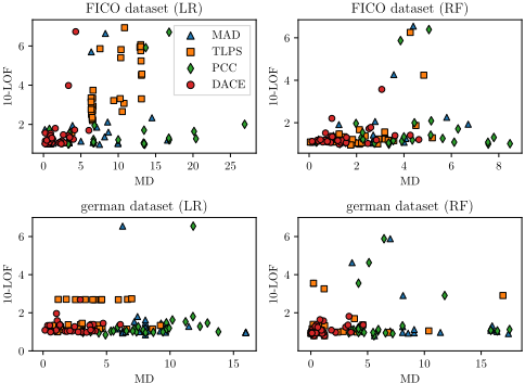
We compared the actions extracted by DACE with ones by the baselines. We set λ = 1.0 for the FICO dataset and λ = 0.01 for the german dataset, respectively. These parameters are selected based on the sensitivity analyses described below. Table 3 presents the average MD, 10-LOF, and running time for each classifier and dataset, and shows that DACE achieved lower MD and 10-LOF than those of the baselines methods regardless of classifiers and datasets. These results suggest that DACE obtain more realistic actions than the other baselines do by considering the feature correlation and the risk of leading to an outlier. Regarding the average running time,
λ
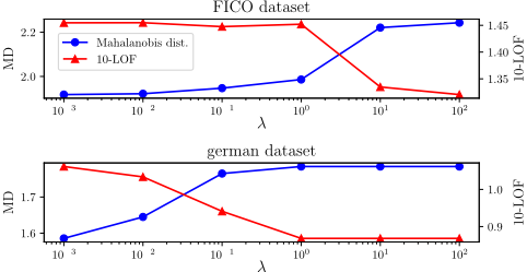
Figure 3: Sensitivity analyses of the trade-off parameter λ of DACE between the average MD and LOF.
DACE was certainly slower than the other baselines. However, Table 3 also indicates that DACE found actions of better quality in terms of both MD and 10-LOF within 600 seconds, which is a reasonable calculation time. Figure 2 presents scatter plots between MD and 10-LOF of each obtained action, and we can see that DACE stably achieved lower MD and 10LOF than the other baselines did. From these results, the effectiveness of DACE has been confirmed in real datasets, and we also argue that our method is favorable when the quality of an action is required by decision-makers and their customers.
5.3 Sensitivity Analysis of Trade-off Parameter
Finally, we show the sensitivity of λ in CDACE on LR classifiers. Figure 3 presents the average MD and 10-LOF of obtained actions a for each λ. We can see that there is a trade-off between MD and LOF of actions obtained by DACE with respect to the value of λ. Consequently, we need to choose λ depending on whether a user emphasizes the preference or reliability of an action. In other words, by varying the value of λ, we can obtain several distinct actions that have diverse characteristics in terms of MD and LOF. As mentioned in [Wachter et al., 2018], suggesting multiple actions may help users for referring to as their future guidelines. Figure 3
indicates that by varying the value of λ, we can obtain several distinct actions that have diverse characteristics in terms of MD and LOF.
6 Conclusion
In this paper, we proposed a new framework of CE for extracting a realistic action by considering the empirical distribution on labeled examples. We introduced a new cost function based on the Mahalanobis' distance (MD) and the local outlier factor (LOF), and then proposed a MILO formulation for optimizing it. By experiments, we confirmed the effectiveness of our method by comparing with existing methods. For future work, there are some directions. First, we plan to devise a more efficient MILO formulation and extend our framework to deal with other classifiers, such as kernel SVMs and deep neural networks. Also, it is interesting to learn the matrix M for MD based on an empirical distribution and a given instance. To clarify when the use of DACE makes more sense, we also plan to conduct further detailed experiments where our assumptions do not hold strongly - e.g., correlations between features are low, etc.
Acknowledgements
We wish to thank Satoshi Hara for making a number of valuable suggestions. We also thank anonymous reviewers for their insightful comments. This work was supported in part by JSPS KAKENHI Grant-in-Aid for Scientific Research (A) 20H00595 and JST CREST JPMJCR18K3.
@inproceedings{ijcai2020p395,
  title     = {DACE: Distribution-Aware Counterfactual Explanation by Mixed-Integer Linear Optimization},
  author    = {Kanamori, Kentaro and Takagi, Takuya and Kobayashi, Ken and Arimura, Hiroki},
  booktitle = {Proceedings of the Twenty-Ninth International Joint Conference on
               Artificial Intelligence, {IJCAI-20}},
  publisher = {International Joint Conferences on Artificial Intelligence Organization},
  editor    = {Christian Bessiere},
  pages     = {2855--2862},
  year      = {2020},
  month     = {7},
  note      = {Main track},
  doi       = {10.24963/ijcai.2020/395},
  url       = {https://doi.org/10.24963/ijcai.2020/395},
}
TY - CPAPER TI - DACE: Distribution-Aware Counterfactual Explanation by Mixed-Integer Linear Optimization AU - Kanamori, Kentaro AU - Takagi, Takuya AU - Kobayashi, Ken AU - Arimura, Hiroki T2 - Proceedings of the Twenty-Ninth International Joint Conference on Artificial Intelligence, IJCAI-20 PB - International Joint Conferences on Artificial Intelligence Organization PY - 2020 SP - 2855 EP - 2862 DO - 10.24963/ijcai.2020/395 UR - https://doi.org/10.24963/ijcai.2020/395 ER -Copied
Machine-readable versions of this paper, for tools and AI agents:





