On Computational Complexity of Pickup-and-Delivery Problems with Precedence Constraints or Time Windows

1 Introduction and Background

General Pickup-and-Delivery Problems (PD) consider routing vehicles to pick up passengers/goods from different origins and delivery them to different destinations with various constraints including for example time windows or precedence constraints being satisfied [Parragh et al., 2008; Battarra et al., 2014; Doerner and Salazar-Gonz´alez, 2014; Dumas et al., 1991; Baldacci et al., 2011]. The problems are important variants of Vehicle Routing Problems (VRP) [Toth and Vigo, 2014], which have been well studied as one of the central combinatorial optimization problems for decades in Operations Research. PD problems are of considerable relevance to AI research, in areas including for examples, planning and scheduling [Beck et al., 2003]; automatous robotics [Gini, 2017; Nunes et al., 2017]; multi-agent systems [Vokˇr´ınek et al., 2010; Coltin and Veloso, 2014; Maciejewski et al., 2017], and constraints satisfaction [Shaw, 1998; Bent and Van Hentenryck, 2007a; Bent and Van Hentenryck, 2007b]. With the rising popularity in the recent years of ridesharing and drivesharing services, PDs are of increasing importance towards building up intelligent transportation network systems for several AI initiatives such as smart cities [Bistaffa et al., 2015; Yao et al., 2018].

Despite the importance and relevance of VRP/PD problems, very limited work has been dedicated specifically in evaluating computational complexities of restricted classes/variants of these problems. Considering VRP/PDs themselves are generalizations to Traveling Salesman Problems, assumptions on NP-hardness of VRP/PD restricted variants in many cases should hold, that is, usually one does not have to worry about that these problems could actually be polynomial-time solvable.

Expectedly all exact algorithms for solving VPR/PD problems with optimality (which have been developed in the past and are mostly based on traditional Operations Research techniques such as branch-and-cut, Bender's decomposition, or mixed integer linear programming) are limited in their scalability [Cordeau, 2006; Hern´andez-P´erez and SalazarGonz´alez, 2009]. In general, instances with sizes greater than 100 in the number of total customers/cities could not be solved optimally; A phenomenon empirically supports the validity of the assumption on intractability of these problems. For the sake of practicality, a wide variety of heuristics have been proposed and developed to this end, including the ones, for examples, based on meta-heuristics, tabu search, local search, genetic search, and their hybridizations [Gendreau et al., 1994; Potvin and Bengio, 1996; Taillard et al., 1997; Br¨aysy and Gendreau, 2005; Laporte et al., 2006] It indeed works fairly well that, when all exact algorithms for a given a VRP/PD problem are not scalable, heuristic solutions are to be sought alternatively. Nevertheless, in an order to justify applications of any heuristics, we owe a "yes" answer to the basic question associated with the problem: Is the problem really NP-hard?

Complexities of many classical AI problems (such as planning, Bayesian networks and theirs probabilistic inferences) have been extensively studied, with multiple dividing lines on tractability delineated successfully [Bylander, 1994; Dean and Boddy, 1988; Cooper, 1990; Blum and Rivest, 1988]. Availability of a set of boundary intractable cases enables convenient generalizations of complexity results. For example, given a new problem A, if we know A is a general version problem to NP-hard problem B, we know right away that A is also NP-hard. Because of this derived fact of NPhardness of A, it is justified developing heuristics for A.

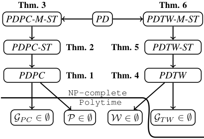
We believe complexities of PDs deserve systematic studies in their own rights. In this paper, we define PDPC/PDTW(vehicle routing Pickup-and-Delivery problems with Precedence Constraints, or Time Windows). PDPC (PDTW) consists of a set of tasks which can be represented as a connected graph G, and a set of Precedence Constraints P (a set of Time Windows W) on these tasks. Starting and finishing at the depot, a vehicle with unit capacity in PDPC (PDTW) needs to figure out a permutation of tasks which satisfies both G and P (or W). Key and critical complexity-theoretic results obtained in this research are: We show both PDPC and PDTW are NPcomplete and they are boundary cases, meaning a relaxation of either G or P/W leads to tractability of the problem (see Figure 8 in the conclusion section for further reference).

We move on to investigate the source of intractability in PDPCs. Specifically we first propose a local search model, whose effectiveness are empirically verified. Using the model as a solver for sets of randomly generalized PDPC instances, we are able to allocate phase transition from solvability to unsolvability, which in turn enables us to pinpoint sources of computational intractability in both the topology and size of the cities, and in the size of precedence constraints to PDPC problems. We believe the formalism can act as a base for developing a full-fledged practical PDPC solver, and the results we obtained on computational hardness and on the sources contributing to this hardness will shed light to a better understanding of PDPC/PD, both in theory, and in development of practical PDPC/PD solvers.

The remainder of the paper is organized as follows. Section 2 presents definitions and complexity results. Possible source on intractability is investigated and analyzed empirically in Section 3. A local search for PDPC is also proposed in the same section. The paper is concluded in Section 4.

2 NP-Completeness of PDPC and PDTW

In this section, we first define PDPC/PDTW (vehicle routing Pickup-and-Delivery problems with Precedence Constraints, or Time Windows) and their various variants in Section 2.1. NP-Completeness theorems are provided next in Section 2.2.

2.1 Definitions

Definitions in this section are grouped into two categories: on Precedence Constraints, and on Time Windows 1 .

1 For our own research purpose, problems in this section are all defined around the computational tractability boundaries. Nevertheless, general versions of PDs can be easily found in the literature, for example, [Toth and Vigo, 2014], [Savelsbergh and Sol, 1995], and

Definition 1 (PDPC) A vehicle routing Pickup-and-Delivery problem with Precedence Constraints is defined with respect to a 2-tuple Θ = 〈G, P〉 where

• G = (C, T, depot) is a directed graph and specifically, C is the set of vertices (corresponding to cities), T is the set of edges (corresponding to tasks). For example, if we have (ci, cj) ∈ T, a one-unit entity (passenger, package, commodity, etc.) needs to be picked up from ci and delivered to cj, and depot ∈ C, which is the city where the vehicle starts/finishes;
• Set P consists of precedence constraints applied on T. That is, for example, if we have ti, tj ∈ T and [ti ≺ tj] ∈ P, it is required that ti should occur before tj.

Given a unit-capacity vehicle, does there exist a single path from and finishing at the depot such that all tasks in T are executed, with all precedence constraints in P satisfied?

Definition 2 (PDPC-ST) PDPC-ST is a variant to PDPC, with the depot city in PDPC replaced by cs, the starting city of the vehicle, and ct, the finishing city of the vehicle. Given a unit-capacity vehicle, does there exist a single path from cs to ct such that all tasks in T are executed, with all precedence constraints in P satisfied?

Definition 3 (PDPC-M-ST) PDPC-M-ST is a variant to PDPC. In the problem, there are m vehicles with m starting cities and m finishing cities. Given m unit-capacity vehicles, do there exist m paths for each of the m vehicle (say ith ) to start at cis and to finish at cit ? In the end all tasks in T are executed, with all precedence constraints in P satisfied.

Definition 4 (PDTW) A vehicle routing Pickup-andDelivery problem with Time Windows is defined with respect to a 2-tuple 〈G,W〉 where

• G = (C, T, depot) is defined the same as the G in PDPC.
• In addition W is a set of time-window constraints applied on T. That is, for example, if we have t ∈ T and [t, τi, τj] ∈ W, it is required that task t should occur between the time τi and τj.

Definition 5 (PDTW-ST) Same problem as PDPC-ST, but P in PDPC-ST is replaced by W in PDTW-ST.

Definition 6 (PDTW-M-ST) Same problem as PDPC-MST, but P in PDPC-M-ST is replaced by W in PDTW-M-ST.

2.2 Complexity Results

Several NP-completeness results are presented in this section. For brevity, proof for Theorem 1 only is elaborated.

Theorem 1 PDPC is NP-complete.

Proof: NP-hardness of PDPC is proved by a polytime transformation from the NP-complete Directed Hamiltonian Circuit Problem (DHC) to PDPC. Figure 1 is an example DHC. From an instance digraph G, we need to create Θ, an instance of PDPC. We use the example in Figure 1 as the running example to help explain the transformation.

[Parragh et al., 2008].

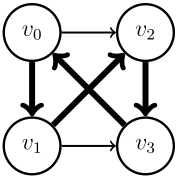
Note 1): A DHC 〈v0, v1, v2, v3, v0〉 is highlighted with thick lines.

Note 2): DHC is listed as [GT38] in [Garey and Johnson, 1979].

Figure 1: A Directed Hamiltonian Circuit in G = (V, E)

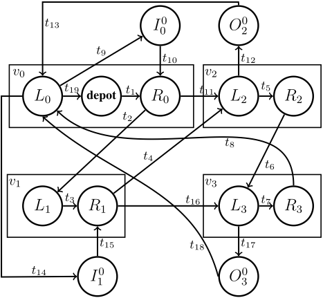
For each vertex vi ∈ V of G, we create two cities Li and Ri in the set C of G. Each vertex v thus corresponds to exactly one dotted rectangle in Figure 2. (Rectangle v0 further includes a depot node, to be explained soon.) Each rectangle boxes two cities, one left and one right. Inside each box, there is a task leaving the left city and entering the right city. If there is an edge leaving vi in G, there is a corresponding task that leaving the city Ri in G. Similarly, if there is an edge entering vi in G, there is a corresponding task entering the city Li in G.

Each edge e ∈ E of G corresponds to a task t in TE, and TE ⊂ T. We need to add additional in-cites and out-cities wherever the in-degree and the out-degree of a city in G are not equal. In the example, these cities are R0, R1, L2 and L3. Accordingly, we add city I 0 0 which enters R0, I 0 1 enteringR1, O0 2 which leaves L2, and O0 3 leaving L3.

We continue with the step of creating the depot: Without loss of generality, we pickup rectangle v0. We add the depot between L0 and R0. As shown in Figure 2, instead of entering city R0 directly, city L0 now enters the depot, and then the depot enters R0. The set TV consists of all tasks linking left cities to right cities in the rectangles. For rectangle v0 however, there are two tasks (L0, depot) and (depot,R0). In Figure 2 for example, TV consists of five tasks {t1, t3, t5, t7, t19}. TV is also a subset of T; To make sure the existence of an Euler Tour in G, we need further a step of balancing the degrees of the in-cities and the outcities: We first pick up the left city in the same rectangle of the depot city. In the case of Figure 2, it is L0. L0 will enter all the in-cites, and all the out-cites will enter L0.

Figure 2 corresponds to G = (C, T, depot), which is created from the input graph G = (V,E). The set C is a union of left cities, right cities, the depot, in-cities, and out-cities. Define TB as the set of all tasks that need to enter/leave the in/out cities (Subscript "B" in TB refers to Balancing degrees for cities in G). The set T is thus a union of TV , TE and TB, i.e., T ≡ TV ∪TE ∪TB. Size of T in Figure 2 is 19, referring to all tasks to be accomplished by the only vehicle. All tasks in Figure 2 are labeled.

We now specify the precedence constraint P. Let the only task leaving depot be t1 and the only task entering it be t|T| (in Figure 2, t|T| is t19). T reduced V ≡ Tv - t1 - t|T|, consisting of all left-city-to-right-city tasks. P asks that t1 precedes, and t|T| is preceded by T reduced V . Further, it is required that T reduced V precedes all tasks in TB, and TB precedes t|T|. Formally P is defined as 2

In the example of Figure 2, we have P in the form of

Transformation is complete. PDPC is in NP, as it is easy to verify if a given task sequence completes all tasks with precedence constraints being followed. For the NP-hardness part we prove that there exists a DHC in a graph G iff a vehicle starting from the depot can accomplish all tasks in G and returns to the depot in the end, with all precedence constraints in P satisfied.

(⇒): If there exists a DHC E′ ⊆ E where G = (V,E), E′ corresponds to a sequence of tasks Tdhc starting from the depot to city L0. The vehicle is one task ((L0, depot) = t|T|) away from the depot. Task t|T | can not be achieved right away because precedence constraints require that all tasks in TB need to be achieved before t|T|. Note that in general some, but not all, tasks in TE are included in Tdhc. In the example, Tdhc is a sequence of [t1, t2, t3, t4, t5, t6, t7, t8]. Tasks {t2, t4, t6, t8} ⊂ TE are in Tdhc. Tasks {t11, t16} ⊂ TE however are not included in Tdhc. But the vehicle at L0 can always achieve a task to enter an in-city and then enter a rectangle to achieve one of the so-far unachieved tasks in TE before it arrives at the corresponding out-city and returns back to L0. In the example, we achieve task t11 with a sequence of [t9, t10, t11, t12, t13], and we achieve task t16 with a sequence of [t14, t15, t16, t17, t18]. Finally the vehicle achieves task t19. Note that no precedence constraints are violated with this sequence. Since we have a DHC

2 Note that the two tasks, t1 and t|T|, do not have to be included in P for the proof to work. As a result, the hight of P (i.e., the size of the longest chains in P) is bounded by 2.

〈v0, v1, v2, v3, v0〉 in G, we end up obtaining a sequence of tasks [t1, t2, t3, . . . , t17, t18, t19] in Θ(G).

(⇐): Suppose there exists a sequence of tasks T in Θ(G) starting and finishing both at the depot. The first task t1 in T must be (depot, R0) and the last task t|T | must be (L0, depot). All tasks in TV other than t|T| must be achieved before any task in TB, because T follows the precedence constraints P. Hence in T , when the vehicle first time arrives at L0, the path it has explored to the point must be a DHC in G. □

Theorem 2 PDPC-ST is NP-complete.

Proof Sketch: It is easier to prove NP-hardness of PDPCST directly from PDPC. The depot in an instance of PDPC is replaced in transformation by the starting point depots and the finishing point depott in the resulting instance of PDPDST. All tasks that initially leave the depot now leave depots . All tasks that initially arrive at the depot now arrive at depott . There exists a completion of tasks from the depot to the depot iff there exists a completion from depots to depott . □

We can obtain further the following (the proof is skipped):

Theorem 3 PDPC-M-ST is NP-complete.

The following three complexity results are related to time windows.

Theorem 4 PDTW is NP-complete.

Proof Sketch: Transformation in proving NP-completeness of PDPC can be repeated here basically. Precedence constraints set P defined as

in PDPC however need to be replaced by a W. In this W, we only need to introduce three time points τ1, τ2, and τ3 such that τ1 < τ2 < τ3, and we require that t1 occurs before τ1; All tasks in T reduced V occur between τ1 and τ2; All tasks in TB occur between τ2 and τ3; and t|T | occurs after τ3. There exists a DHC in a graph G iff a vehicle starting from the depot accomplishes all tasks in G of PDTW and returns to the depot in the end, with W satisfied. □

We can obtain further the following (proofs skipped):

Theorem 5 PDTW-ST is NP-complete.

Theorem 6 PDTW-M-ST is NP-complete.

3 Analysis on Computational Hardness

In this section, we present the local search approach for solving PDPC. First, we introduce the algorithm in Section 3.1. We then perform empirical analysis to test the effectiveness of this new local search approach in Section 3.2. Finally in Section 3.3, local search is used as a solver to investigate sources contributing to the hardness of PDPC problems.

3.1 A Local Search for PDPC

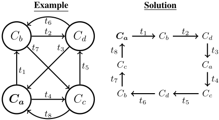
We use Figure 3 as a PDPC example instance to help explain concepts. The example has four cities from Ca to Cd in C and the depot is city Ca. There are eight tasks in T from t1 up to t8. The precedence constraints P ≡ {t2 ≺ t3; t2 ≺ t6; t4 ≺ t8}. Obviously permutation [t1, t2, . . . , t7, t8] serves as a solution to the problem (also shown in Figure 3).

Algorithm 1: A Local Search for PDPC

Input: 〈G, P〉, an instance of PDPC, where

G = (C, T, depot).

Output: Toutput, a permutation of all tasks in T of G;

and the cost c associated with Toutput.

• 1 Initialization: Set cost c to its maximal possible value; Set threshold value for maximal rounds maxRound; And create a random permutation Toutput;
• 2 while (c > 0 or maxRound not reached) do
• 3 Check each task t ∈ T for every alternative position p in the current permutation Toutput; If there are positions where c value can be reduced, update Toutput by moving t to the position that yields greatest c value reduction; Update c accordingly;

4 end

A high level algorithmic description of using local search for solutions to PDPC is provided in Algorithm 1. Details more related to implementation are skipped here in the interest of brevity for a focus on key ideas. Necessary explanation to the algorithm however is presented as follows.

Given a PDPC instance, the algorithm starts from a random permutation of tasks Toutput, which is associated with a cost c. Up to maxRound rounds of local search, for a repeatedly revised task sequence Toutput with gradually reduced c value, are to be performed. Of course after each iteration, if c = 0 is achieved, it means that a solution to the problem - an Euler Tour starting from and finishing at the depot with all precedence constraints satisfied - is found. As a result, the algorithm will break the loop and return Toutput. For each round, each task t is considered once, for its optimal position p with mostly reduced c value. After the round, task t is moved to position p to update both Toutput and c, which are the inputs for the next loop, if c remains to be greater than 0.

Note that size of the local-search neighbourhood is bounded by the total number of tasks. As indicated in Algorithm 1, the task in investigation tries all candidate positions, if a better one is found, the task is removed from its current position and inserted into the new position.

We now discuss a few important issues must be taken into consideration for Algorithm 1 to actually work. First, how

1

2

3

4

5

6

7

8

Figure 4: A random permutation of eight tasks

a permutation of tasks is represented? We can simply use a conceptually circular array consisting of |T| elements/tasks, with an awareness that if the sequence is an Euler Tour, any two neighbouring tasks should be connected by a city, and the first and the last task in the array should be connected too, by the depot city. If a permutation of tasks in the array is a Euler Tour to G, and a linear extension to P, the permutation is a solution to the PDPC problem Θ = 〈G,P〉, subject further to the fact that the first task starts from the depot. For example, the permutation of tasks in Figure 5 offers an alternative solution to the PDPC problem in Figure 3.

But how the cost of a permutation is decided? In our model, the cost is a weighted summation over three parts

where c1 = 1, if the task on position one is not from the depot, c1 = 0 otherwise; c2 is the total number of nonneighboring tasks in the permutation; And c3 is the total number of precedence constraints in P violated. Weights are set to w1 = w2 = w3 = 1. Figure 4 is an example random permutation. It's cost is 8 = 1 + 5 + 2. That is, task t3 is not from the depot, and there are five violations of neighborhood requirements as specified in G of Figure 3. Regarding precedence constraints, only (t4 ≺ t8) ∈ P holds. To reduce the cost, we need to perform local search on better position for the task being evaluated. If one such position is found, we just remove the task from its current position, and insert it into the new position. Other tasks get affected will only need to move either all left, or all right. Circular movement of tasks are not necessary, and position 1 will be more likely holding a task that is actually from the depot, as local search converges to a solution when they exist. It can be verified that in Figure 4, if we move task t1 to position 1, tasks t3, t5, t6, t7, and t2 need to move one position to their right respectively, and the total cost is reduced from 8 to 6, We then move task t2 to position 2, the total cost is further reduced from 6 to 2. Task t3 to position 6, and task t5 to position 5, resulting in the permutation in Figure 5. Finally, when there are equal choices of tasks movements, we choose a random one. We do not adopt any other trap escaping strategy except for random starts if the algorithm can not get out of a local minimum after a threshold number of non-improvement rounds.

3.2 Empirical Evaluation on Local Search

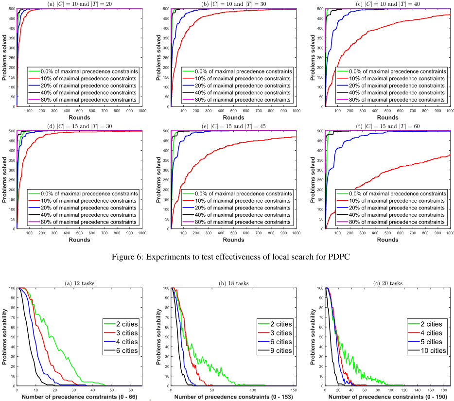
In this section, we test the effectiveness of the proposed local search using six sets of randomly generated data (corresponding respectively to the six subfigures in Figure 6). Each set is characterized by two measures, |C| the total number of cities in an instance, and |T| the total number of tasks.

Let k = |T|, we know that the range of total possible number of precedence constraints are from 0 to maximal k(k - 1)/2. For each set, we consider five different cases where a range of 0.0%, 10%, 20%, 40%, 80% of maximal total possible precedence constraints are considered. Hence we have five curves in different colors for these five cases in each one of the sub-figures in Figure 6. For each case we create 500 random examples 3 using 500 different random seeds. Each example allows up to 1000 rounds to solve. After n rounds (where n equals the total number of tasks) noimprovement encountered, local search creates another random Euler Tour, and continue. Observations from these experiments are as follow.

Effectiveness. The local search formalism proposed here, and the cost function designed as the sum of violated number of connectedness and precedence of tasks, can actually be used as heuristics to guide the search, leading to finding of a solution with a reasonable searching efforts. With exception to the red cases (the ones having 10% of precedence constraints), almost all problem instances can be solved in less than 300 rounds. Note that we do not adopt any strategy for escaping local minima, because current research focus on the work has been dedicated to carrying out a qualitative evaluation on the effectiveness and efficiency of the local search, instead of developing an off-the-shelf PDPC solver).

Presence of precedence. When comparing the 5 curves in any sub-figure (i.e., comparing different extents of precedence constraints on task, it is obvious that all green problems can be solved in ten rounds for all six sets. Since they are not constrained on precedence, local search actually deals with Euler Tour finding, for which we know that polynomial algorithms exist. When the problems are constrained to 10% precedence (red curves), local search becomes greatly slower in convergence to all problems, i.e., approaching the ceiling. When the ratios are further increased to 20%, and 40% (blue problems and black problems, respectively), the problems become easier and easier to solve, indicated by the fact that the curves are raised higher earlier, meaning it takes fewer rounds to solve. For almost all the magenta problems, they can be solved within 1-2 rounds. This fast convergence phenomenon is explainable: Considering that magenta problems are highly constrained on precedence, a linear extension is almost there. Given that we have the guarantee on solvability of these problems, it means that the linear extension, whihc is shaped almost completely by these 80% precedence constraints, is actually the solution to the PDPC problems.

Time efficiency. In Figure 6, from left to right, from the first row, to the second row, the problem size is getting larger, with the total rounds kept the same to 1000. For the red problems, this becomes somewhat problematic, as less and less of them can actually be solved while we know beforehand that solutions to the problems exist. This is supposed to be happening when we are using a poly-time complete algorithm to tackle NP-complete problems (assuming P!=NP). Note that our local search is a complete solver to PDPC in the sense that through random restarts a solution to a given problem instance can always be found by the approach as long as it exists. How long it takes or how many random starts are needed is a separate concern.

3 Examples are with guarantee on existence of solutions.

3.3 Sources Contributing to PDPCHardness

From Figure 6, it appears that the real computational hardness for PDPCs occurs more likely around those 10% regions. Accordingly we perform another theme of experiments, which are dedicated to investigating sources that contribute to PDPC hardness. For these experiments, we use the local search model as a complete solver to PDPC problems, which means, if a PDPC instance is solvable, the procedure will find it within the given maximal round. This assumption is reasonable, should we feed local search only problems comparatively smaller in size (e.g., 1000 rounds maximal is apparently enough for those 30 tasks cases (b) and (d) subfigures in Figure 6); We use two different random permutations to generate Euler Tour and precedence constraints for creating a random PDPC instance 4 .

We consider three different experimental groups, where the total number of cities equals to 12, 18, and 20 respectively. For each group, we further consider four cities, which correspond to four different-color curves in each one of the three sub-figures in Figure 7. Again when the size of tasks |T | = k is given, maximal possible precedence constraints can be calculated using k(k - 1)/2. For k = 12, 18, 20, the values are 66, 153, and 190, respectively, corresponding to horizontal axis in Figure 7. Given k, for each precedence constraint value p ∈ [0, k(k -1)/2], we create 100 random PDPC problem instances for each one of the four different cities. Results obtained from these experiments are pictorially illustrated in Figure 7. Below is our main observations on PDPC hardness.

When PDPC problem instances are very lightly constrained by precedences (when the number of constraints is less than 10 or so), almost all PDPC problems are solvable. In case they are heavily constrained (rule of thumbs, when the number of constraints is greater than 40% or 60%), all PDPC problems are unsolvable; Putting this argument to the extreme: When there is no precedence constraints, PDPC is reduced to finding an Euler Tour, and all the problem instances are solvable, and when there is full precedence constraints, order of tasks are constrained into a specifical linearization, which, almost impossible, coincides with the Euler tour permutation of tasks.

Although transitions between solvability and solvability phases in Figure 7 are not rapid, difficult problem instances however do occur around transition regions, where about 50% of the problem instances are solvable. For example, the most computationally challenging case for sub-figure-a in Figure 6 (10 cities and 20 tasks) is the one with 10% constraints. At the same time, the black curve in sub-figure-c of Figure 7 (corresponding to 10 cities and 20 tasks too) makes phase transition on solvability between 1 to 30 precedence constraints, and 19 = 190 × 10% falls in this region.

4 Different from instances generated in Section 3.2, we no longer have the guarantee on the solvability of these problem instances.

Drawing a vertical cut on the four curves with a given number of precedence constraint within the transition region, it is always the case from top to bottom in the color: green, red, blue and black. This necessarily implies that, accordingly to this observation, for two PDPC problems constrained by the same number of precedence constraints, the problem with more cities are more likely to be unsolvable. Hence we conclude that both size and topology of G affect the solvability of PDPC problems.

Similarly, drawing a horizontal cut on the four curves at the y-axis point 50 (meaning 50% of the problems are solved), the cut will cross the curves in the order of black, blue, red, and green, meaning that for a given number of tasks, for PDPC problems with more cities, fewer precedence constraints are needed to reach the computationally difficult region of PDPC problems.

4 Conclusions and FutureWork

This paper contributes to a better understanding of computational properties of the vehicle routing PD problems. It shows several highly restricted variants of PD (including PDPC and PDTW) are NP-complete. To our best knowledge, these complexity results are the first ones of the kind. The results justify applications of heuristic methods for any problem which is a general version of either PDPC or PDTW. After all, it makes less sense, for approaching a problem using approximation or heuristics without knowing that the problem is indeed computationally intractable in the first place.

Complexity results are summarized in Figure 8 pictorially, where an arrow connects a problem to its restricted version. An interesting computational tractability line is delineated in the figure. With Pickup-and-delivery only (i.e., P or W is empty) PDPC/PDTW equals to the polytime-solvable problem of finding an Euler Tour in G; With precedence constraints only (i.e., GPC ∈ ∅), PDPC equals to the poly-time problem of topological sorting on tasks. With both P and GPC, PDPC is NP-complete. However for PDTW, with W alone (i.e., GTW ∈ ∅), the problem remains NP-hard: It is easy to constrain n tasks with Allen's Interval Algebra (IA) [Allen, 1983] in terms of time windows; And it is well known Satisfiability for Allen's IA is NP-complete [Vilain and Kautz, 1986].

As noted previously in the proof, the transformation for proving Theorem 1 can be used to obtain NP-hardness of PDPC where the height of P is bounded by 2. Also, it is noted that the Directed Hamiltonian Circuit Problem serves as the core problem in reductions in the NP-hardness proofs for Temporal Projection Problems [Tan and Gruninger, 2009; Tan, 2012] and for the Partial-Order Plan Viability Problems [Tan and Gruninger, 2014]. Further restriction on either G or P will eventually land us into tractable zones. For example, we conjecture that, 1) when GPC is bounded by in-degree=out-degree=2, or 2) when P is further restricted with topological structures such as N-free or seriesparallel [M¨ohring, 1989], PDPC would become poly-time solvable. Complexity results on Allen's IA are comprehensive in the literature, where all maximal subalgebra for Allen's IA have been identified [Nebel and B¨urckert, 1995;

Krokhin et al., 2003]. Since W in the proof for Theorem 4 is obviously a tractable subalgebra of Allen's (it just includes the operator "before"), we have in addition the following research question - a restricted version of PDTW, where time windows for tasks are restricted to certain maximal subalgebra of Allen's IA, is polytime solvable.

A local search-based model has been proposed in this paper to find solutions for PDPC problems. Using it as a complete PDPC solver, we investigated the possible sources leading to the intractability of PDPC, through studying on how phase transition from solvability to unsolvability with increasing precedence constraints. Local search has long been used as a tool in tackling NP-hard problems [Johnson et al., 1988]. Some motivating examples are [Savelsbergh, 1985], [Minton et al., 1992] and [Vaessens et al., 1996]. While we believe local-search encodings other than the one proposed in the paper will also serve our research well, the current approach is straightforward and rather simple - we take the benefit of defining the total number of costs as simply a weighted sum of violated constraints.

A recent research effort looked into the relationships between problem difficulty, phase transition, heuristic search, and cost-based heuristics [Cohen and Beck, 2017b; Cohen and Beck, 2017a]. Particularly in [Cohen and Beck, 2017b], an analytical framework for investigating the phase transition in heuristic search is proposed. Evaluating the applicability of this abstract model to the analysis of the local search for PDPC, would be an interesting line of future work.

Since our main purpose is to make fair comparisons between problem instances on total rounds necessary to find a solution, efforts have yet to be taken in turning up the model for optimized performance. For future work, standard local minimum escaping techniques such as Discrete Lagrangian Method [Shang and Wah, 1998] might be further incorporated into the model as necessary. We are also considering encoding PDPC problems as propositional satisfiability problems [Gomes et al., 2008; Pham et al., 2008]. The objective seems to be within a reasonably quick reach, given the CSP (constraint satisfaction problem) nature of these problems.

Finally, it should be interesting to make use of these new insights on intractability of PDPC to test benchmarks generally used in the literature, and to investigate their applicability on real-world domains such as Uber trips, or robots deployments in Amazon fulfillment and distribution centers.

Acknowledgments

We are grateful to all the anonymous reviewers for their insightful feedback and detailed suggestions. This research was supported by a Discovery Grant from the Natural Sciences and Engineering Research Council of Canada (NSERC), an Ontario Research Fund-Research Excellence award in BRAIN Alliance, and the York Research Chairs (YRC) program. The first author is additionally supported by a Research Fellow Opportunity Grant from the Social Sciences and Humanities Research Council of Canada (SSHRC).