
CFM: Convolutional Factorization Machines for Context-Aware Recommendation
Proceedings of the Twenty-Eighth International Joint Conference on Artificial Intelligence. Main track. Pages 3926-3932.
https://doi.org/10.24963/ijcai.2019/545
Keywords
- Multidisciplinary Topics and Applications: Recommender Systems
- Machine Learning: Recommender Systems
- Machine Learning: Learning Preferences or Rankings
Abstract
Factorization Machine (FM) is an effective solution for context-aware recommender systems (CARS) which models second-order feature interactions by inner product. However, it is insufficient to capture high-order and nonlinear interaction signals. While several recent efforts have enhanced FM with neural networks, they assume the embedding dimensions are independent from each other and model high-order interactions in a rather implicit manner. In this paper, we propose Convolutional Factorization Machine (CFM) to address above limitations. Specifically, CFM models second-order interactions with outer product, resulting in ''images'' which capture correlations between embedding dimensions. Then all generated ''images'' are stacked, forming an interaction cube. 3D convolution is applied above it to learn high-order interaction signals in an explicit approach. Besides, we also leverage a self-attention mechanism to perform the pooling of features to reduce time complexity. We conduct extensive experiments on three real-world datasets, demonstrating significant improvement of CFM over competing methods for context-aware top-k recommendation.
- [Baltrunas et al., 2015] Linas Baltrunas, Karen Church, Alexandros Karatzoglou, and Nuria Oliver. Frappe: Understanding the usage and perception of mobile app recommendations in-the-wild. arXiv preprint arXiv:1505.03014, 2015.
- [Bayer et al., 2017] Immanuel Bayer, Xiangnan He, Bhargav Kanagal, and Steffen Rendle. A generic coordinate de- scent framework for learning from implicit feedback. In WWW, pages 1341-1350, 2017.
- [Beutel et al., 2018] Alex Beutel, Paul Covington, Sagar Jain, Can Xu, Jia Li, Vince Gatto, and Ed H Chi. Latent cross: Making use of context in recurrent recommender systems. In CIKM, pages 46-54. ACM, 2018.
- [Chen et al., 2012] Tianqi Chen, Weinan Zhang, Qiuxia Lu, Kailong Chen, Zhao Zheng, and Yong Yu. Svdfeature: a toolkit for feature-based collaborative filtering. JMLR Journal, 13(Dec):3619-3622, 2012.
- [Cheng et al., 2016] Heng-Tze Cheng, Levent Koc, Jeremiah Harmsen, Tal Shaked, Tushar Chandra, Hrishi Aradhye, Glen Anderson, Greg Corrado, Wei Chai, Mustafa Ispir, et al. Wide & deep learning for recom- mender systems. In Proceedings of the 1st Workshop on Deep Learning for Recommender Systems, pages 7-10. ACM, 2016.
- [Duchi et al., 2011] John Duchi, Elad Hazan, and Yoram Singer. Adaptive subgradient methods for online learning and stochastic optimization. JMLR Journal, 12(Jul):2121- 2159, 2011.
- [Guo et al., 2017] Huifeng Guo, Ruiming Tang, Yunming Ye, Zhenguo Li, and Xiuqiang He. Deepfm: A factorization-machine based neural network for ctr predic- tion. In IJCAI, 2017. IJCAI
- [Hahnloser et al., 2000] Richard HR Hahnloser, Rahul Sarpeshkar, Misha A Mahowald, Rodney J Douglas, and H Sebastian Seung. Digital selection and analogue amplification coexist in a cortex-inspired silicon circuit. Nature, 405(6789):947, 2000.
- [He and Chua, 2017] Xiangnan He and Tat-Seng Chua. Neu- ral factorization machines for sparse predictive analytics. In SIGIR, pages 355-364. ACM, 2017.
- [He et al., 2016a] Kaiming He, Xiangyu Zhang, Shaoqing Ren, and Jian Sun. Deep residual learning for image recog- nition. In CVPR, pages 770-778, 2016.
- [He et al., 2016b] Kaiming He, Xiangyu Zhang, Shaoqing Ren, and Jian Sun. Identity mappings in deep residual networks. In ECCV, pages 630-645. Springer, 2016.
- [He et al., 2017] Xiangnan He, Lizi Liao, Hanwang Zhang, Liqiang Nie, Xia Hu, and Tat-Seng Chua. Neural collabo- rative filtering. In WWW, pages 173-182, 2017.
- [He et al., 2018a] Xiangnan He, Xiaoyu Du, Xiuli Wang, Feng Tian, Jinhui Tang, and Tat-Seng Chua. Outer product-based neural collaborative filtering. In IJCAI, 2018. IJCAI
- [He et al., 2018b] Xiangnan He, Zhankui He, Jingkuan Song, Zhenguang Liu, Yu-Gang Jiang, and Tat-Seng Chua. Nais: Neural attentive item similarity model for recom- mendation. TKDE, 30(12):2354-2366, 2018.
- [Järvelin and Kekäläinen, 2002] Kalervo Järvelin and Jaana Kekäläinen. Cumulated gain-based evaluation of ir tech- niques. TOIS, 20(4):422-446, 2002.
- [Koren et al., 2009] Yehuda Koren, Robert Bell, and Chris Volinsky. Matrix factorization techniques for recom- mender systems. Computer, pages 30-37, 2009.
- [Rendle et al., 2009] Steffen Rendle, Christoph Freuden- thaler, Zeno Gantner, and Lars Schmidt-Thieme. Bpr: Bayesian personalized ranking from implicit feedback. In UAI, pages 452-461. AUAI Press, 2009.
- [Rendle, 2010] Steffen Rendle. Factorization machines. In ICDM, pages 995-1000, 2010.
- [Rendle, 2012] Steffen Rendle. Factorization machines with libfm. TIST, 3(3):57, 2012.
- [Shan et al., 2016] Ying Shan, T Ryan Hoens, Jian Jiao, Hai- jing Wang, Dong Yu, and JC Mao. Deep crossing: Web- scale modeling without manually crafted combinatorial features. In SIGKDD, pages 255-262. ACM, 2016.
- [Wang et al., 2017] Ruoxi Wang, Bin Fu, Gang Fu, and Min- gliang Wang. Deep & cross network for ad click predic- tions. In Proceedings of the ADKDD'17, page 12. ACM, 2017.
- [Wang et al., 2018] Xiang Wang, Xiangnan He, Fuli Feng, Liqiang Nie, and Tat-Seng Chua. Tem: Tree-enhanced em- bedding model for explainable recommendation. In WWW, pages 1543-1552, 2018.
- [Wu et al., 2019] Libing Wu, Cong Quan, Chenliang Li, Qian Wang, Bolong Zheng, and Xiangyang Luo. A context-aware user-item representation learning for item recommendation. TOIS, 37(2):22, 2019.
- [Xiao et al., 2017] Jun Xiao, Hao Ye, Xiangnan He, Han- wang Zhang, Fei Wu, and Tat-Seng Chua. Attentional factorization machines: Learning the weight of feature in- teractions via attention networks. In IJCAI, pages 3119- 3125, 2017. IJCAI
- [Yuan et al., 2016] Fajie Yuan, Guibing Guo, Joemon M. Jose, Long Chen, Haitao Yu, and Weinan Zhang. Lambdafm: Learning optimal ranking with factorization machines using lambda surrogates. In CIKM, pages 227- 236, 2016.
- [Zhang et al., 2014] Yongfeng Zhang, Guokun Lai, Min Zhang, Yi Zhang, Yiqun Liu, and Shaoping Ma. Explicit factor models for explainable recommendation based on phrase-level sentiment analysis. In SIGIR, pages 83-92. ACM, 2014.
- [Zhou et al., 2018] Guorui Zhou, Xiaoqiang Zhu, Chenru Song, Ying Fan, Han Zhu, Xiao Ma, Yanghui Yan, Junqi Jin, Han Li, and Kun Gai. Deep interest network for click- through rate prediction. In SIGKDD, pages 1059-1068. ACM, 2018.
References were extracted automatically from the PDF and may contain errors.
Full text extracted automatically from the PDF; figures, tables and equations may differ. The PDF is the version of record.
1 Introduction
Recommender system serves as an effective tool to predict user behaviors, such as click/purchase on products, having been extensively used in practical applications. When characterizing user behavior data, besides the most essential information of user ID and item ID, rich context information is also available. Examples of contexts include but are not limited to user demographics, item attributes, time/location of the current transaction, historical records and the information of last transactions [Bayer et al., 2017; Wu et al., 2019]. To learn from such context-rich data, a universal solution is to first convert it into high-dimensional generic feature vectors (e.g., by using one-hot/multi-hot encoding on univalent/multivalent categorical variables) [Zhou et al., 2018], and then build predictive models on the featured inputs [He and Chua, 2017]. Distinct from continuous realvalued features that are naturally found in images and audios, the featured inputs of CARS are mostly categorical, resulting in high-dimensional yet sparse feature vectors. This poses difficulties to build predictive models, such that traditional supervised learning solutions such as SVMs and deep neural networks are sub-optimal and less efficient, since they are not tailored for learning from sparse data.
∗The co-first authors contribute equally.
To design effective models for CARS, the key ingredient is to account for the interactions among features [Wang et al., 2017]. Existing solutions to feature interaction modeling can be categorized into two types:
1. Manually constructing cross features. This type of methods manually construct combinatorial features, which explicitly encode feature interactions. Then the cross features are fed into predictive models such as logistic regression [Cheng et al., 2016] and deep neural networks [Wang et al., 2018]. Apparently, the cross feature construction process requires heavy engineering efforts and domain knowledge, making the solution less adaptable to other domains. In addition, another drawback is that it cannot generalize to cold-start feature interactions that are unseen in training data.
2. Automatically learning feature interactions. This type of methods learn feature interactions and their effects in a unified model. A typical paradigm is to associate each feature with an embedding, expressing the feature interaction as a function over feature embeddings. For example, FM [Rendle, 2010] models the interaction of two features as the inner product of their embeddings, and Deep Crossing [Shan et al., 2016] concatenates feature embeddings and feeds them into a multi-layer perceptron (MLP) to learn high-order interactions. However, these methods implicitly assume embedding dimensions are independent from each other, which goes against the semantics of latent dimensions [Zhang et al., 2014] and limits the model expressiveness. Moreover, MLP over embedding concatenation captures feature interactions in a rather implicit manner, which has been manifested inefficient to model multiplicative relations [Beutel et al., 2018].
In this paper, we focus on developing methods for CARS with the aim of addressing the above-mentioned drawbacks of existing solutions. To reduce engineering efforts in constructing cross features, we explore embedding-based methods and propose Convolutional Factorization Machine (CFM) which automatically learns feature interactions. More precisely, feature embeddings are firstly fed to a self-attention pooling layer, which can dramatically reduce the computational cost and debilitate the influence of noisy features. Then, we model second-order interactions with outer product, resulting in a list of 2D matrices, which is more effective to capture correlations between embedding dimensions compared with inner product. After that we stack the generated matrices and obtain a 3D interactions cube that encodes all second-order interactions. To explicitly learn high-order signals, we propose to employ 3D convolution on the interaction cube, stacking a multi-layer 3D convolution neural network (CNN) above it. As a result, CFM addresses the major limitations of stateof-the-art CARS methods - independent embedding dimensions and implicit high-order interaction modeling. The main contributions of this work are as follows:
- We propose to utilize an interaction cube to represent feature interactions, which encodes both interaction signals and embedding dimension correlations.
- We propose to employ 3D CNN above the interaction cube, which can effectively capture high-order interactions in an explicit way. To the best of our knowledge, this is the first attempt to explore 3D CNN in feature interaction modeling.
- We leverage a self-attention mechanism to perform pooling operations for features, reducing computational time complexity.
- We conduct comprehensive experiments on publicly accessible datasets to comparatively evaluate and demonstrate the effectiveness of the proposed method.
2 Preliminaries
Factorization Machine [Rendle, 2010; Rendle, 2012] is a generic framework which integrates the advantages of flexible feature engineering and high-accuracy prediction of latent factor models. In FM, every transaction is represented by a multi-field categorical feature vector x ∈ Rm which utilizes one-hot/multi-hot encoding to depict contextual information. An example is illustrated as follows with three feature fields.
The scoring function of FM is defined as
where w0 represents the global bias, wi represents the bias factor for the i-th variable. The pairwise interaction of feature xi and xj is captured by a factorized parametrization 〈vi, vj〉 = ∑df=1 vif vjf , where 〈·, ·〉 denotes the inner product of two vectors. vi ∈ Rd can be seen as the embedding vector for feature xi.
Besides, Eq.(1) can be reformulated, resulting in linear time complexity O(md) which makes FM applicable and efficient [Rendle, 2010]. However, the major drawback of FM is that it only models the second-order feature interactions in a linear way 1 , which is insufficient to learn complex (i.e., nonlinear and high-order) signals from real-world data. Although several recent efforts have enhanced FM with neural networks, like NFM [He and Chua, 2017] and DeepFM [Guo et al., 2017], they assume the embedding dimensions are independent from each other and model high-order interactions in a rather implicit manner.
3 Convolutional FactorizationMachine
In this section, we present the details and the training procedure of the proposed CFMmodel. We also analyze the relationship between CFM and some other similar research. Before diving into the technical details, we first introduce some basic notations.
Throughout the paper, we use bold uppercase letter (e.g., M) to denote a matrix, bold lowercase letter to denote a vector (e.g., x), and calligraphic uppercase letter to denote a 3D tensor (e.g., C). Scalar is represented by lowercase letters (e.g., y). The target of CFM is to generate a ranked item list for a given user context.
3.1 The CFMModel
It can been seen from Eq.(1) that the original FM only accounts for second-order feature interactions in a linear way by inner product, which fails to learn complex signals. To address this problem, the prediction rule of CFM is formulated as Eq.(2):
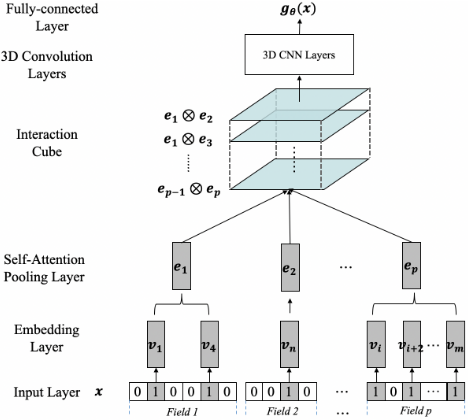
where gθ(x) denotes the core component to model feature interactions. In the following parts, we will elaborate how to learn gθ(x) by outer product and 3D CNN, which explicitly captures high-order interaction signals. Figure 1 illustrates the overall structure of the proposed CFMmodel.
Input and Embedding Layer
The input layer is fed with a sparse contextual vector x, which may contain both one-hot features (e.g., userID) and multihot features (e.g., historical items) to describe a specific user context and item attributes. Then each feature xi is projected into a d-dimensional dense vector representation vi ∈ Rd by the embedding layer. Due to the sparsity of x, we only need to consider the non-zero features (i.e., xi ̸= 0). This can be easily achieved through an embedding table lookup.
Self-Attention Pooling Layer
In the real-world scenario, the number of non-zero features in x may be very large, especially with various of multi-hot features (e.g., historical items). The original time complexity to account for all pairwise feature interactions is O(m2 ). Then, FM utilizes a reformulation to rewrite Eq.(1) and makes the time complexity to be linear with m. However, the involved reformulation can only suit for inner product.
Compared with the large number of features, it's obvious that the number of fields is much smaller. As a result, another solution to reduce computational cost is to perform the pooling operation on features and learn a single embedding for each field. Intuitive approaches include max-pooling and average-pooling. However, we argue that this kind of methods is sub-optimal due to the lack of learning process. To capture the intuition that different features have varying importance, we propose to use an attention mechanism to compute the importance of each feature and perform the pooling operation.
1 Although FM has high-order formulations [Rendle, 2010], it still belongs to linear models and is proved to be difficult to estimate.
Suppose the set of non-zero features in field j is Xj, we parameterize the attention score of feature xi ∈ Xj with a MLP, which is defined as
where Wj and bj are corresponding weight matrix and bias vector that project the input embedding into a hidden state, and hTj is the vector which projects the hidden state into the attention score. The size of hidden state is termed as "attention factor". Then, the importance of xi is calculated by normalizing the attention score through the softmax function:
Finally, the after-pooling embedding ej for field j is formulated as
In fact, the self-attention pooling layer not only reduces the computational cost but also debilitates the influence of noisy features and redundant feature interactions.
Interaction Cube
After the pooling layer, we propose to use a 3D interaction cube to represent feature interactions. Specifically, the interaction between ei and ej is modeled by an outer product operation between them, as shown in Eq.(6).
The above d×d matrix can be seen as a two-dimensional "image" which contains both interaction signals and embedding dimension correlations. Suppose the contextual vector x contains p feature fields, the total number of generated "images" is p(p - 1)/2. All these "images" are stacked to form a 3D tensor C which is the input of the following 3D CNN.
The major advantage of using this cube to represent feature interactions lies in the following points:
- The outer product matrix is more effective to capture dimension correlations compared with conventional inner and element-wise product, which assume that embedding dimensions are independent with each other.
- The 3D structure provides an explicit solution to model high-order interactions, which can be seen as interactions between different "floors" of this cube. For example, in Figure 1, the interaction between the first floor (e1 ⊗ e2) and the second floor (e1 ⊗ e3) can be considered as a third-order interaction among e1, e2 and e3.
- The 3D format also provides a good input for the well developed 3D CNN. While it's designed for capturing sequential patterns, its 3D architecture can also benefit the modeling of high-order interactions, which can be regarded as convolutions in the depth direction.
3D Convolution Layers
In order to tackle with the 3D interaction cube and extract signals more effectively, a multi-layer 3D CNN is applied to learn feature interaction patterns 2 . It can be abstracted as
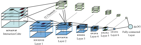
Suppose the embedding size d = 64 and the number of feature fields p = 10, the size of the interaction cube is 64 × 64 × 45. Figure 2 illustrates the structure of the stacked 3D CNN with 6 hidden layers, where each hidden layer has 32 channels and convolution operations are performed in all three directions (i.e., width, height and depth).
2 Although multi-channel 2D CNN can also be used to process the interaction cube, the 3D CNN is a more effective approach. Experimental results are shown in the following part.
In each layer, we first perform 3D convolutions between a 3D kernel and the input cube, after which we add a bias and perform a nonlinear transformation by using ReLU [Hahnloser et al., 2000] as the activation function to obtain a new output cube. It's obvious that the convolution in the depth direction captures high-order feature interactions in a rather explicit manner. According to Figure 2, the filter shape in the first layer is [2,2,14] and the stride is [2,2,1], which is corresponding to width, height and depth. In the subsequent layers, the filter shape and stride are both [2,2,2].
The output of the 3D convolution layers is a vector g. After that, we adopt a fully-connected layer to re-weight each dimension of g and calculate a real-valued scalar as gθ(x):
3.2 Training Details
The focus of CFM is generating top-k recommendation other than rating prediction. Therefore, we optimize the proposed CFM model with the BPR framework [Rendle et al., 2009]:
where x- is the sampled negative transaction corresponding to the positive one x+, and σ is the sigmoid function. More detailly, we first sample a mini-batch of positive user-item transactions (i.e., x+), which contain feature vectors to describe specific user contexts and item attributes. Thereafter, for every specific user context, negative items are randomly sampled from a uniform distribution. Then we combine the features of the sampled negative items and the corresponding user context features to form negative user-item transactions (i.e., x-). Finally, both positive and negative transactions are fed to train the loss function defined in Eq.(10). Recent works have demonstrated that an adaptive sampling distribution would result in better performance [Yuan et al., 2016], while it's not the focus of this work. We leave this exploration as future work.
The embedding layer is pre-trained with FM using BPR loss. To avoid overfitting, we involve L2 regularization on the embedding layer, convolution layers and the fully-connected layer. Besides, before the final fully-connected layer, a dropout layer is also inserted.
3.3 Discussion
Time Complexity
As described above, the depth of the interaction cube is p(p1)/2. Given the embedding size d, the time complexity to perform 3D convolution is O(p2d2 ). Given the situation that p ≪ m, we can see that the major complexity comes from d2 which is introduced by the convolution. However, this burden can be largely reduced through GPU acceleration.
The other part of complexity comes from feature pooling. Assume the attention factor is n, the time complexity to calculate attention is O(mnd). Therefore, the total time complexity of CFM is O(p2d2 + mnd).
Relationship with Other Models
Neural factorization machine (NFM) [He and Chua, 2017] is also proposed to address the linearity problem of FM. It introduces a MLP to learn high-order and nonlinear signals. However, NFM is still based on inner product and MLP is a rather implicit approach to capture high-order signals. Besides, MLP is also much harder to train because of the need of more parameters and even suffers from detrimental performance when the network goes deeper [He and Chua, 2017].
| Dataset | #users | #items | #transactions | #fields |
|---|---|---|---|---|
| Frappe | 957 | 4,082 | 96,203 | 10 |
| Last.fm | 1,000 | 20,301 | 214,574 | 4 |
| MovieLens | 6,040 | 3,665 | 939,809 | 4 |
Attention factorization machine (AFM) [Xiao et al., 2017] is proposed to enhance FM by assigning different attentions to different feature interactions. However, the major purpose of attention mechanism in CFM is to perform feature pooling and reduce computational cost. Besides, we argue that the importance of feature interactions is automatically learned through the convolution procedure of CFM.
Another related research is ONCF [He et al., 2018a], which improves matrix factorization (MF) [Koren et al., 2009] through outer-product. The main difference between ONCF and CFM is that ONCF is based on MF but CFM is motivated from FM. From this perspective, the relationship between CFM and ONCF is something like the relationship between FM and SVDFeature [Chen et al., 2012].
4 Experiments
In this section, we conduct experiments with the aim of answering the following research questions:
RQ1: Does CFM model outperform state-of-the-art methods for CARS top-k recommendation?
RQ2: How do the special designs of CFM (i.e., interaction cube and 3DCNN) affect the model performance?
RQ3: What's the effect of the attention-based feature pooling?
4.1 Experimental Settings
Data Description
To evaluate the performance of the proposed CFM model, we conduct comprehensive experiments on three real-world implicit feedback datasets: Frappe 3 , Last.fm 4 and MovieLens 5 . Table 1 summarizes the statistics of these datasets.
Frappe. This dataset is conducted by [Baltrunas et al., 2015] to generate right app recommendations for right moments. Frappe contains 96, 203 app usage logs of different user contexts. Each log contains 10 contextual feature fields (i.e., p = 10) including user ID, item ID, daytime and some other information.
Last.fm. The Last.fm dataset is for music recommendation. We extract the latest one day listening history of 1,000 users. The user context is described by user ID and the last music ID that the user has listened within 90 minutes. The item attributes include music ID and artist ID.
3 http://baltrunas.info/research-menu/frappe
4 http://www.dtic.upf.edu/ ocelma/MusicRecommendationDataset
5 https://grouplens.org/datasets/movielens/latest/
MovieLens. The original MovieLens dataset is designed for explicit rating prediction. Here we binarize it into implicit feedback. The user context is described by user ID and historical items (multi-hot). The item feature is composed of movie ID and movie genres (multi-hot).
Evaluation Protocols
We adopt the leave-one-out evaluation to test the performance of models, which has been widely used in literature [He et al., 2017; Yuan et al., 2016; He et al., 2018b]. More specifically, for Last.fm and MovieLens, the latest transaction of each user is held out for testing and the remaining data is treated as the training set. For the Frappe dataset, because there is no timestamp information so we randomly select one transaction for each specific user context as the test example.
The recommendation quality is evaluated by Hit Ratio (HR) and Normalized Discounted Cumulative Gain (NDCG). HR@k is a recall-based metric, measuring whether the test item is in the top-k positions of the recommendation list (1 for yes and 0 otherwise). NDCG@k are weighted versions which assign higher scores to the top-ranked items [J¨arvelin and Kek¨al¨ainen, 2002].
Baselines
We implemented CFM 6 using TensorFlow. We compare the performance of CFM with the following baselines:
- PopRank: This method returns top-k most popular items. It acts as a basic benchmark.
- FM: The original factorization machine [Rendle, 2010] trained by BPR loss [Rendle et al., 2009].
- NFM: Neural factorization machine [He and Chua, 2017] is a strong baseline which uses a MLP to learn nonlinear and high-order interaction signals.
- DeepFM: This method [Guo et al., 2017] ensembles the original FM and a MLP to generate recommendation.
- ONCF: This method [He et al., 2018a] is a newly proposed algorithm which improves MF with outer product.
Parameter Settings
To fairly compare the performance of models, we train all of them by optimizing the BPR loss with mini-batch Adagrad [Duchi et al., 2011]. The learning rate is searched between [0.01,0.02,0.05] for all models. The batch size is set as 256. For all models except PopRank and FM, we pretrain them using the original FM with 500 iterations. The dropout ratio for NFM, DeepFM, ONCF, and CFM is tuned in [0.1,0.2,···,0.9]. The embedding size and attention factor is set as 64 and 32, respectively. The output channels of CNNbased models (i.e., ONCF and CFM) are set as 32. Regarding NFM, the number of MLP layers is set as 1 with 64 neurons, which is the recommended setting of their original paper [He and Chua, 2017]. For the deep component of DeepFM, we set the MLP according to their original paper [Guo et al., 2017], which has 3 layers and 200 neurons in each layer.
6 Codes are available at https://github.com/chenboability/CFM
Because the number of feature fields p differs between different datasets, the sizes of interaction cubes are also different, resulting in different kernel sizes and strides of 3D convolution layers 7 . More specifically, we use the structure illustrated in Figure 2 on the Frappe dataset. For Last.fm and MovieLens, the filter shape is [2,2,2] and the stride is [2,2,1] for all six layers.
4.2 Performance Comparison (RQ1)
Table 2 shows the top-k recommendation performance on all three datasets. It's obvious that CFM achieves the best performance on all datasets regarding to both HR and NDCG. We argue that this significant improvement lies in the following basements: 1) The outer product-based interaction cube is a fairly good approach to represent feature interactions. This can be seen from the comparison between CFM and NFM, which uses inner product-based pooling vectors to present feature interactions. 2) The involved 3D CNN is more effective to extract signals compared with 2D CNN (ONCF) and MLP (NFM, DeepFM), especially for high-order interactions.
Among the baselines, we can see that both NFM and DeepFM achieve better performance than original FM. The reason is that they involve MLP to learn nonlinear and highorder interaction signals. However, their methods are too implicit and MLP is also harder to train compared with the local connected CNN.
4.3 Model Investigation (RQ2)
Study of the Interaction Cube
To further demonstrate the effectiveness of interaction cube, we convert it to a 2D feature map through two different operations. The former is to tile the generated matrices (i.e., Mi,j) to form a bigger feature map (tiled) 8 . The latter is to perform a max pooling operation on its depth direction (pooling). Then we use a 6-layers 2D CNN to learn signals from the map. Figure 3a shows the results on Frappe. We can see that CFM achieves better performance than the tiled method. The reason is the stacked 3D architecture provides a rather explicit approach to model high-order interactions. Besides, we can also see that the max pooling operation will definitely downgrade the performance because it only considers the most important information. However, the performance is still better than the original FM, which demonstrates the effectiveness of outer product and the strong learning capability of CNN.
Study of 3D CNN
To tackle with the 3D interaction cube, another solution is to use multi-channel 2D CNN (MCNN). Here, we also conduct experiments to make a comparison between them. Figure 3b illustrates the results on the Frappe dataset. We can see that compared with MCNN, our CFM achieves better performance. The reason is that the convolution in the depth direction of 3DCNN explicitly models high-order feature interactions while MCNN cannot achieve this in such an explicit manner.
7 Another approach is to use padding so that the settings of CNN layers can be fixed.
8 For Frappe, the size of feature map is 320×576 = 64×64×45.
| HR | Frappe | Last.fm | Movielens | ||||||
|---|---|---|---|---|---|---|---|---|---|
| HR@5 | HR@10 | HR@20 | HR@5 | HR@10 | HR@20 | HR@5 | HR@10 | HR@20 | |
| PopRank | 0.2539 | 0.3493 | 0.4136 | 0.0013 | 0.0023 | 0.0032 | 0.0121 | 0.0235 | 0.0429 |
| FM | 0.4204 | 0.5486 | 0.6590 | 0.1658 | 0.2382 | 0.3537 | 0.0512 | 0.0998 | 0.1762 |
| DeepFM | 0.4632 | 0.6035 | 0.7322 | 0.1773 | 0.2612 | 0.3799 | 0.0563 | 0.1170 | 0.2033 |
| NFM | 0.4798 | 0.6197 | 0.7382 | 0.1827 | 0.2676 | 0.3783 | 0.0634 | 0.1192 | 0.2029 |
| ONCF | 0.5359 | 0.6531 | 0.7691 | 0.2183 | 0.3208 | 0.4611 | 0.0579 | 0.1110 | 0.2002 |
| CFM∗ | 0.5462 | 0.6720 | 0.7774 | 0.2375 | 0.3538 | 0.4841 | 0.0697 | 0.1323 | 0.2248 |
| NDCG | Frappe | Last.fm | Movielens | ||||||
| NG@5 | NG@10 | NG@20 | NG@5 | NG@10 | NG@20 | NG@5 | NG@10 | NG@20 | |
| PopRank | 0.1595 | 0.1898 | 0.2060 | 0.0007 | 0.0011 | 0.0013 | 0.0071 | 0.0107 | 0.0156 |
| FM | 0.3054 | 0.3469 | 0.3750 | 0.1142 | 0.1374 | 0.1665 | 0.0295 | 0.0452 | 0.0644 |
| DeepFM | 0.3308 | 0.3765 | 0.4092 | 0.1204 | 0.1473 | 0.1772 | 0.0355 | 0.0526 | 0.0723 |
| NFM | 0.3469 | 0.3924 | 0.4225 | 0.1235 | 0.1488 | 0.1765 | 0.0374 | 0.0553 | 0.0748 |
| ONCF | 0.3940 | 0.4320 | 0.4614 | 0.1493 | 0.1823 | 0.2176 | 0.0343 | 0.0514 | 0.0738 |
| CFM∗ | 0.4153 | 0.4560 | 0.4859 | 0.1573 | 0.1948 | 0.2277 | 0.0426 | 0.0627 | 0.0858 |
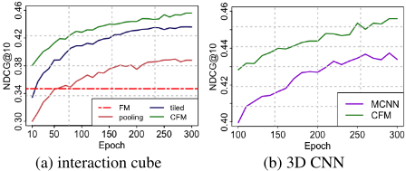
Figure 3: Study of interaction cube and 3D CNN
4.4 Study of Feature Pooling (RQ3)
The proposed CFM leverages a self-attention mechanism to perform feature pooling. To demonstrate the effectiveness of the involved attention mechanism, we replace it with maxpooling and mean-pooling. Table 3 shows the results on MovieLens. We can see that mean-pooling achieves better performance than max-pooling because max-pooling only considers the most important feature and lots of information is discarded. However, the attention-based CFM achieves the best performance. In fact, the attention-based feature pooling automatically assigns different importance to different features. It can not only retain the rich feature information but also debilitate the noise influence.
Table 4 shows the comparison between CFM with and without feature pooling on MovieLens dataset. We can see that the attention-based feature pooling can dramatically reduce the training time without affecting the model performance. It can even result in better recommendation quality.
5 Conclusion
In this work, we propose a novel context-aware recommendation algorithm CFM, which seamlessly combines automatic feature interaction modeling of FM and strong learning capability of 3D CNN. The key design of CFM is to use an outer product-based interaction cube to represent feature interactions and then utilize 3D CNN to extract signals from it. As a result, correlations among embedding dimensions can be effectively captured and higher-order interaction signals can also be learned in a rather explicit approach. Besides, we also utilize a self-attention mechanism to perform feature pooling and reduce computational cost. Extensive experiments on three datasets demonstrate that CFM has superior performance compared with state-of-the-art models when generating top-k recommendation. Future work includes using more advanced techniques, such as residual learning [He et al., 2016a; He et al., 2016b], to better extract signals. Besides, we are also interested in developing more rational methods to further improve the efficiency of CFM.
| Model | HR@10 | HR@20 | NG@10 | NG@20 |
| Max | 0.1257 | 0.2142 | 0.0591 | 0.0813 |
| Mean | 0.1291 | 0.2212 | 0.0603 | 0.0833 |
| CFM | 0.1323 | 0.2248 | 0.0627 | 0.0858 |
| Indicator | FM | CFM | CFM-wfp |
|---|---|---|---|
| Time(min) | 0.53 | 4.63 | 50.52 |
| HR@10 | 0.0998 | 0.1323 | 0.1297 |
| NG@10 | 0.0452 | 0.0627 | 0.0605 |
Acknowledgements
This research is funded by the project: E-commerce and public service platform of modern arts, Shanghai. Dong Wang and Joemon Jose are corresponding authors.
@inproceedings{ijcai2019p545,
  title     = {CFM: Convolutional Factorization Machines for Context-Aware Recommendation},
  author    = {Xin, Xin and Chen, Bo and He, Xiangnan and Wang, Dong and Ding, Yue and Jose, Joemon},
  booktitle = {Proceedings of the Twenty-Eighth International Joint Conference on
               Artificial Intelligence, {IJCAI-19}},
  publisher = {International Joint Conferences on Artificial Intelligence Organization},
  editor    = {Sarit Kraus},
  pages     = {3926--3932},
  year      = {2019},
  month     = {8},
  note      = {Main track},
  doi       = {10.24963/ijcai.2019/545},
  url       = {https://doi.org/10.24963/ijcai.2019/545},
}
TY - CPAPER TI - CFM: Convolutional Factorization Machines for Context-Aware Recommendation AU - Xin, Xin AU - Chen, Bo AU - He, Xiangnan AU - Wang, Dong AU - Ding, Yue AU - Jose, Joemon T2 - Proceedings of the Twenty-Eighth International Joint Conference on Artificial Intelligence, IJCAI-19 PB - International Joint Conferences on Artificial Intelligence Organization PY - 2019 SP - 3926 EP - 3932 DO - 10.24963/ijcai.2019/545 UR - https://doi.org/10.24963/ijcai.2019/545 ER -Copied
Machine-readable versions of this paper, for tools and AI agents:





