
SynthNet: Learning to Synthesize Music End-to-End
Proceedings of the Twenty-Eighth International Joint Conference on Artificial Intelligence. Main track. Pages 3367-3374.
https://doi.org/10.24963/ijcai.2019/467
Keywords
- Machine Learning: Interpretability
- Machine Learning: Deep Learning
- Machine Learning: Time-series;Data Streams
- Machine Learning: Learning Generative Models
- Multidisciplinary Topics and Applications: Art and Music
Abstract
We consider the problem of learning a mapping directly from annotated music to waveforms, bypassing traditional single note synthesis. We propose a specific architecture based on WaveNet, a convolutional autoregressive generative model designed for text to speech. We investigate the representations learned by these models on music and concludethat mappings between musical notes and the instrument timbre can be learned directly from the raw audio coupled with the musical score, in binary piano roll format.Our model requires minimal training data (9 minutes), is substantially better in quality and converges 6 times faster in comparison to strong baselines in the form of powerful text to speech models.The quality of the generated waveforms (generation accuracy) is sufficiently high,that they are almost identical to the ground truth.Our evaluations are based on both the RMSE of the Constant-Q transform, and mean opinion scores from human subjects.We validate our work using 7 distinct synthetic instrument timbres, real cello music and also provide visualizations and links to all generated audio.
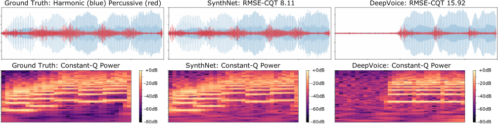
- SynthNet: Constant-Q Power SynthNet: RMSE-CQT 8.11 DeepVoice: Constant-Q Power DeepVoice: RMSE-CQT 15.92
- Ground Truth: Constant-Q Power Ground Truth: Harmonic (blue) Percussive (red) References [Arik et al., 2017]
- Sercan O Arik, Mike Chrzanowski, Adam Coates, Gregory Diamos, Andrew Gibiansky, Yongguo Kang, Xian Li, John Miller, Andrew Ng, Jonathan Raiman, et al. Deep voice: Real-time neural text-to-speech. arXiv preprint arXiv:1702.07825, 2017.
- [Briot et al., 2017] Jean-Pierre Briot, Gaëtan Hadjeres, and François Pachet. Deep learning techniques for music generation-a survey. arXiv preprint arXiv:1709.01620, 2017.
- [Brown, 1991] Judith C Brown. Calculation of a constant q spectral transform. The Journal of the Acoustical Society of America, 89(1):425-434, 1991.
- [Chollet, 2017] François Chollet. Xception: Deep learning with depthwise separable convolutions. arXiv preprint, pages 1610-02357, 2017.
- [Dieleman et al., 2018] Sander Dieleman, Aäron van den Oord, and Karen Simonyan. The challenge of realistic music generation: modelling raw audio at scale. arXiv preprint arXiv:1806.10474, 2018.
- [Donahue et al., 2018] Chris Donahue, Julian McAuley, and Miller Puckette. Synthesizing audio with generative adver- sarial networks. arXiv preprint arXiv:1802.04208, 2018.
- [Engel et al., 2017] Jesse Engel, Cinjon Resnick, Adam Roberts, Sander Dieleman, Douglas Eck, Karen Simonyan, and Mohammad Norouzi. Neural audio synthesis of mu- sical notes with wavenet autoencoders. arXiv preprint arXiv:1704.01279, 2017.
- [Gatys et al., 2015] Leon A Gatys, Alexander S Ecker, and Matthias Bethge. A neural algorithm of artistic style. arXiv preprint arXiv:1508.06576, 2015.
- [Howard et al., 2017] Andrew G Howard, Menglong Zhu, Bo Chen, Dmitry Kalenichenko, Weijun Wang, Tobias Weyand, Marco Andreetto, and Hartwig Adam. Mobilenets: Efficient convolutional neural networks for mobile vision applications. arXiv preprint arXiv:1704.04861, 2017.
- [Kingma and Ba, 2014] Diederik P Kingma and Jimmy Ba. Adam: A method for stochastic optimization. arXiv preprint arXiv:1412.6980, 2014.
- [Klambauer et al., 2017] Günter Klambauer, Thomas Un- terthiner, Andreas Mayr, and Sepp Hochreiter. Self- normalizing neural networks. In Advances in Neural Infor- mation Processing Systems, pages 971-980, 2017.
- [Maaten and Hinton, 2008] Laurens van der Maaten and Ge- offrey Hinton. Visualizing data using t-sne. Journal of machine learning research, 9(Nov):2579-2605, 2008.
- [Mehri et al., 2016] Soroush Mehri, Kundan Kumar, Ishaan Gulrajani, Rithesh Kumar, Shubham Jain, Jose Sotelo, Aaron Courville, and Yoshua Bengio. Samplernn: An unconditional end-to-end neural audio generation model. arXiv preprint arXiv:1612.07837, 2016.
- [Mor et al., 2018] Noam Mor, Lior Wolf, Adam Polyak, and Yaniv Taigman. A universal music translation network. arXiv preprint arXiv:1805.07848, 2018.
- [Sethares, 2005] William A Sethares. Tuning, timbre, spec- trum, scale. Springer Science & Business Media, 2005.
- [Theis et al., 2015] Lucas Theis, Aäron van den Oord, and Matthias Bethge. A note on the evaluation of generative models. arXiv preprint arXiv:1511.01844, 2015.
- [Thickstun et al., 2016] John Thickstun, Zaid Harchaoui, and Sham Kakade. Learning features of music from scratch. arXiv preprint arXiv:1611.09827, 2016.
- [Van Den Oord et al., 2016] Aäron Van Den Oord, Sander Dieleman, Heiga Zen, Karen Simonyan, Oriol Vinyals, Alex Graves, Nal Kalchbrenner, Andrew Senior, and Koray Kavukcuoglu. Wavenet: A generative model for raw audio. CoRR abs/1609.03499, 2016.
References were extracted automatically from the PDF and may contain errors.
Full text extracted automatically from the PDF; figures, tables and equations may differ. The PDF is the version of record.
1 Introduction
WaveNets [Van Den Oord et al., 2016] have revolutionized text to speech by producing realistic human voices. Even though the generated speech sounds natural, upon a closer inspection the waveforms are different to genuine recordings. As a natural progression, we propose a WaveNet derivative called SynthNet which can learn and render (in a controlled way) the complex harmonics in the audio training data, to a high level of fidelity. While computer vision is well established, there is little understanding over what audio generative models are learning. Towards enabling similar progress, we give insights into the learned representations of WaveNets, upon which we build our model.
WaveNets were trained using raw audio waveforms aligned with linguistic features. We take a similar approach to learning music synthesizers and train our model based on the raw audio waveforms of entire songs and their symbolic representation of the melody. This is more challenging than speech due to the following differences: 1) in musical compositions multiple notes can be played at the same time, while words are spoken one at a time; 2) the timbre of a musical instrument is arguably more complex than speech; 3) semantically, utterances in music can span over a longer time.
[Van Den Oord et al., 2016] showed that WaveNets can generate new piano compositions based on raw audio. Recently, this work was extended by [Dieleman et al., 2018], delivering a higher consistency in compositional styling. Closer to our work, [Engel et al., 2017] describe a method for learning synthesizers based on individually labelled note-waveforms. This is a laborious task and is impractical for creating synthesizers from real instruments. Our method bypasses this problem since it can directly use audio recordings of an artist playing a given song, on the target instrument.
SynthNet can learn representations of the timbre of a musical instrument more accurately and efficiently via the dilated blocks through depthwise separable convolutions. We show that it is enough to condition only the first input layer, where a joint embedding between notes and the corresponding fundamental frequencies is learned. We remove the skip connections and instead add an additional loss for the conditioning signal. We also use an embedding layer for the audio input and use SeLU [Klambauer et al., 2017] activations in the final block.
The benchmarks against the WaveNet [Van Den Oord et al., 2016] and DeepVoice [Arik et al., 2017] architectures show that our method trains faster and produces high quality audio. After training, SynthNet can generate new audio waveforms in the target timbre, based on a given song which was not seen at training time. While we focus on music, SynthNet can be applied to any time-series domain.
Our contributions are as follows. 1) We show that musical instrument synthesizers can be learned end-to-end based on real and synthetic raw audio and a binary note representation, with minimal training data. Multiple instruments can be learned by a single model, including real instruments (subsection 4.5). 2) We give insights into the representations learned by dilated causal convolutional blocks and consequently propose SynthNet, which provides substantial improvements in quality and training time. Indeed, we demonstrate (Figure 3) that the generated audio is practically identical to the ground truth. 3) The benchmarks against existing architectures contains an extensive set of experiments spanning over three sets of hyperparameters, where we control for the receptive field size. We show that the RMSE of the Constant-Q Transform
(RMSE-CQT) is highly correlated with the mean opinion score (MOS). 4) We find that reducing quantization error via dithering is a critical preprocessing step towards generating the correct melody and learning the correct pitch to fundamental frequency mapping.
2 RelatedWork
In music, style can be defined as the holistic combination of the melodic, rhythmic and harmonic components of a particular piece. The delay and sustain variation between notes determines the rhythmic style. The latter can vary over genres (e.g. Jazz vs Classical) or composers. Timbre or harmonic style can be defined as the short term and steady state (sustained frequency distribution) acoustical properties of a musical instrument [Sethares, 2005]. Our focus is on learning the timbre, while controlling the (given) melodic content and avoiding any rhythmic variations.
The research on content creation is plentiful. For an in depth survey of deep learning methods for music generation we point the reader to the work of [Briot et al., 2017]. Generative autoregressive models were used in [Van Den Oord et al., 2016; Mehri et al., 2016] to generate new random content with similar harmonics and stylistic variations in melody and rhythm. Recently, the work of [Van Den Oord et al., 2016] was extended by [Dieleman et al., 2018] where the quality is improved and the artificial piano compositions are more realistic. We have found piano to be one of the easier instruments to learn. [Donahue et al., 2018] introduce WaveGANs for generating music with rhythmic and melodic variations.
Closer to our work, [Engel et al., 2017] propose WaveNet Autoencoders for learning and merging the harmonic properties of instrument synthesizers. The major difference with our work is that we are able to learn timbres from entire songs (a mapped sequence of notes to the corresponding waveform), while their method requires individually labelled notes (NSynth dataset). With our method, the overhead of learning a new instrument is greatly reduced. Moreover, SynthNet requires minimal data and does not use note velocity.
Based on the architecture proposed by [Engel et al., 2017], and taking a domain adaptation approach, [Mor et al., 2018] condition the generation process based on raw audio. An encoder is used to learn note mappings from a source audio timbre to a target audio timbre. The approach can be more error prone than ours, since it implies the intermediary step of correctly decoding the right notes from raw audio. This can significantly decrease the generation quality. Interestingly, [Mor et al., 2018] play symphonic orchestras from a single instrument audio. However, there is no control over which instrument plays what. Conversely, we use individual scores for each instrument, which gives the user more control. This is how artists usually compose music.
3 End-to-end Synthesizer Learning
[Van Den Oord et al., 2016] and [Arik et al., 2017] have shown that generative convolutional networks effectively learn the human voice from raw audio. This has advanced the state of the art in text to speech (TTS). We further explore the possibilities of these architectures by benchmarking them in the domain of learning music synthesizers. There are considerable differences between the human voice and musical instruments. Firstly, the harmonic complexity of musical instruments is higher than the human voice. Second, even for single instrument music, multiple notes can be played at the same time. This is not true for speech, where only one sound utterance is produced at a time. Lastly, the melodic and rhythmic components in a musical piece span a larger temporal context than a series of phonemes as part of speech. All of these factors make the music domain arguably more challenging than speech.
3.1 Baseline Architectures
Our starting point is the model proposed by [Van Den Oord et al., 2016] with the subsequent refinements in [Arik et al., 2017]. We refer the reader to the these articles for further details. Our data consists of triplets ¶(x1↪ y1↪ z1)↪ ▷ ▷ ▷ ↪ (xN ↪ yN ↪ zS)♦ over N songs and S styles, where xi is the 256-valued encoded waveform, yi is the 128-valued binary encoded MIDI and zs ∈ ¶1↪ 2↪ ▷ ▷ ▷ ↪ S♦ is the one-hot encoded style label. Each audio sample xt is conditioned on the audio samples at all previous timesteps x<t = ¶xt-1↪ xt-2↪ ▷ ▷ ▷ ↪ x1♦, all previous binary MIDI samples and the global conditioning vector. The joint probability of a waveform x = ¶x1↪ ▷ ▷ ▷ ↪ xT ♦ is factorized as follows:
The hidden state before the residual connection in dilation block ℓ is
while the output of every dilation block, after the residual connection is
where τ and σ are respectively the tanh and sigmoid activation functions, ℓ is the layer index, f indicates the filter weights, g the gate weights, r the residual weights and W, V and U are the learned parameters for the main, local conditioning and global conditioning signals respectively. The f and g convolutions are computed in parallel as a single operation [Arik et al., 2017]. All convolutions have a filter width of F . The convolutions with W ℓ and V ℓ are dilated.
To locally condition the audio signal, [Van Den Oord et al., 2016] first up-sample the y time series to the same resolution as the audio signal (obtaining yℓ ) using a transposed convolutional network, while [Arik et al., 2017] use a bidirectional RNN. In our case, the binary midi vector already has the same resolution.
We use an initial causal convolution layer (Equation 4) that only projects the dimension of the signal from 128 channels to the number of residual channels. The first input layers are causal convolutions with parameters W 0 and V 0 for the waveform and respectively the piano roll:
| Input | Dilated conv Skip | Final block | |||||
|---|---|---|---|---|---|---|---|
| Channels | Type | Activation | Separable | Connection | 1x1 Conv | Activation | |
| WaveNet | 1 Scalar | Conv | None | No | Yes | No | ReLU |
| DeepVoice | 256 1-hot | Conv | Tanh | No | Yes | Yes | ReLU |
| SynthNet | 1 Scalar | Embed | Tanh | Yes | No | No | SeLU |
All other architecture related details are kept identical to the ones presented in [Van Den Oord et al., 2016] and [Arik et al., 2017] as best as we could determine. The differences between the two architectures and SynthNet are summarized in Table 1.
We compare the performance and quality of these two baselines against SynthNet initially in Table 3 over three sets of hyperparmeters (Table 2). For the best resulting models we performMOS listening tests, shown in Table 5. Results for global conditioning experiments are provided in Table 4.
3.2 GramMatrix Projections
We perform a set of initial experiments to gain more insight into the learned representations. We use Gram matrices to extract activation statistics since these have been previously used for artistic style transfer[Gatys et al., 2015]. After training, the validation data is fed through five locally conditioned networks, each trained with a distinct timbre.
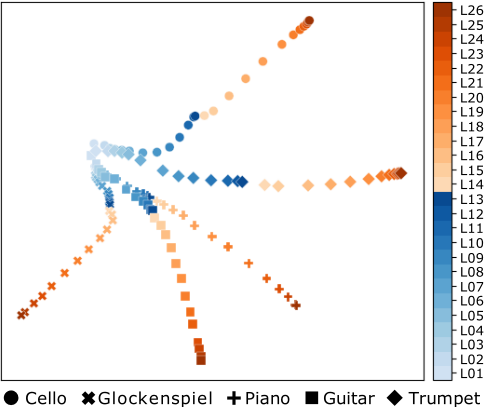
The data has identical melodic content but has different harmonic content (i.e. same song, different instruments). The Gram matrices are extracted from the outputs of each dilated block (Equation 3) for each network - timbre. These are flattened and projected onto 2D, simultaneously over all layers and styles via T-SNE [Maaten and Hinton, 2008]. The results presented in Figure 1 show that the activations separate further as the layer index increases. A broad interpretation is that the initial layers extract low-level generic audio features, these being common to all waveforms.
However, since this is a controlled experiment, we can be more specific. The timbre of a musical instrument is characterized by a specific set of resonating frequencies on top of the fundamental frequency (pure sine wave). Typically one identifies individual notes based on their fundamental, or lowest prominent frequency. These depend on the physics of the musical instrument and effects generated, for example, by the environment. Since the sequence of notes is identical and the timbres differ, we conjectured that Figure 1 could imply a frequency-layer correspondence. While the latter statement might be loose, Gram matrices extracted from the lower layers are nevertheless much closer due the increased similarity with the fundamental frequency.
3.3 SynthNet Architecture
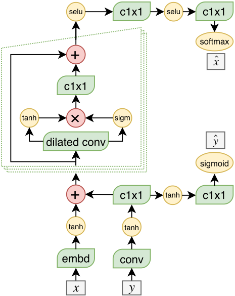
Figure 1 provides indicative results from many experiments. We hypothesize that the skip connections are superfluous and the conditioning of the first input layer should suffice to drive the melodic component. We also hypothesize that the first audio input layer learns an embedding corresponding to the fundamental pitches. Then, we aim to learn mapping from the symbolic representation (binary midi code) to the pitch embeddings (Equation 8). Therefore, in SynthNet there are no parameters learned in each dilation block for local conditioning and the hidden activation with global conditioning (omitted in Figure 2) becomes
The input to the dilated blocks is the sum of the embedding codes and the autoencoder latent codes:
As it can be seen in Figure 2 there are no skip connections and Equation 4 no longer applies. We also found that using SeLU activations [Klambauer et al., 2017] in the last layers improves generation stability and quality. Other normalization strategies could have been used, we found SeLU to work well. In addition, we further increase sparsity by changing the dilated convolution in Equation 6 with a dilated depthwise separable convolution. Separable convolutions perform a channel-wise spatial convolution that is followed by a 1 × 1 convolution.
In our case each input channel is convolved with its own set of filters. Depthwise separable convolutions have been successfully used in mobile and embedded applications [Howard et al., 2017] and in the Xception architecture [Chollet, 2017]. As we show in Table 4 and Table 5, the parsimonious approach works very well since it reduces the complexity of the architecture and speeds up training.
SynthNet is trained with an additional auxiliary autoregressive task on the midi data (y) (see Figure 2). In principle, this allows the model to jointly generate both audio and midi. In practice, the midi part of the model is too simple to generate interesting results. Nonetheless, we found the multitask training beneficial. We conjecture it forces basic midi features to be extracted. In summary, in contrast with Equation 1 we optimize the joint log p(x↪ y♣z), so that
4 Experiments
We compare exact replicas of the architectures described in [Van Den Oord et al., 2016; Arik et al., 2017] with our proposed architecture SynthNet. All are implemented in PyTorch, available at https://github.com/florinsch/synthnet . We train the networks to learn the instrument timbre using raw audio waveforms. The networks are conditioned locally with a 128 binary vector indicating note on-off, extracted from the midi files. The latter describes the melodic content.
For the purpose of validating our hypotheses, we chose to eliminate extra sources of error by manually upsampling the midi files. That is, we simply treat the midi note on/offs as points in continuous time and look up whether the note is on at the given grid point, where the grid may be arbitrarily fine grained. For the results in Table 4, the network is also conditioned globally with a one-hot vector which designates the style (instrument) identity. Hence, multiple instrument synthesizers are learned in a single model. For the hyperparameter search experiments (Table 3) and the final MOS results (Table 5) we train one network for each style, since it is faster. We use the Adam [Kingma and Ba, 2014] optimizer with a batch size of 1, a learning rate of 10-3 , β1 = 0▷9, β2 = 0▷999 and ε = 10-8 with a weight decay of 10-5 . We find that for most instruments 100-150 epochs is enough for generating high quality audio, however we keep training up to 200 epochs to observe any unexpected behaviour or overfitting. All training is done on Tesla P100 GPUs with 16GB of memory.
4.1 Synthetic Registered Audio
We generate the dataset using the freely available Timidity++ 1 software synthesizer. For training we selected parts 2 to 6 from Bach's Cello Suite No. 1 in G major (BWV 1007). We found that this was enough to learn the mapping frommidi to audio and to capture the harmonic properties of the musical instruments. From this suite, the Prelude (since it is most commonly known) is not seen during training and is instead used for measuring the validation loss and for conditioning the generated audio.
After synthesizing the audio, we have approximately 12 minutes of audio for each timbre, of which 9 minutes (75%) is used for training and 3 minutes (25%) for validation. We experiment with S = 7 timbres, which were selected to be as different as possible. Each style corresponds to a specific preset from the 'Fluid-R3-GM' sound font. These are (preset number - instrument): S01 - Bright Yamaha Grand, S09 - Glockenspiel, S24 - Nylon String Guitar, S42 - Cello, S56 - Trumpet, S75 - Pan Flute and S80 - Square Lead.
For training, the single channel waveforms are sampled at 16kHz and the bit-depth is reduced to 8 bit via mu-law encoding. Before reducing the audio bit depth, the waveforms are dithered using a triangular noise distribution with limits (-0▷009↪ 0▷009) and mode 0. This reduces perceptual noise but more importantly keeps the quantization noise out of the signal frequencies, which is critical for the learning process.
Without dithering there are melodic discontinuities and clipping errors in the generated waveforms. The latter errors are most likely due to notes getting mapped to the wrong set of frequencies (artifacts appear due to the quantization error). From all timbres, the added white noise due to dithering is most noticeable for Glockenspiel, Cello and Pan Flute. The midi is upsampled to 16kHz to match the audio sampling rate and each frame contains a 128 valued vector which designates note on-off times for each note (piano roll).
4.2 Measuring Audio Generation Quality
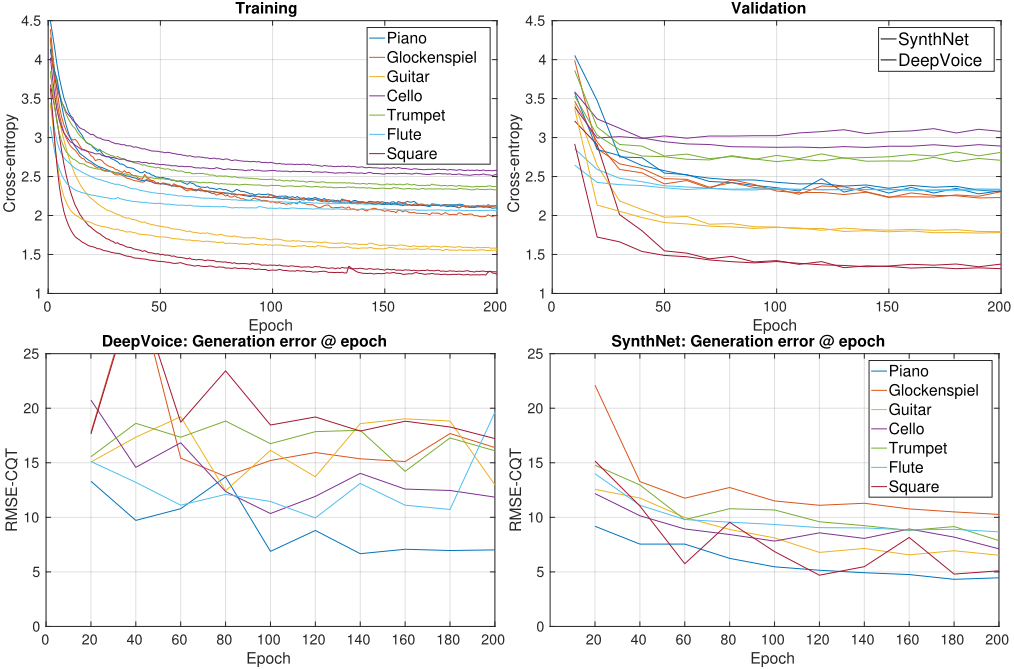
Quantifying the performance of generative models is a nontrivial task. Similarly to [Van Den Oord et al., 2016; Arik et al., 2017] we have found that once the training and validation losses go beyond a certain lower threshold, the quality improves. However, the losses are only informative towards convergence and overfitting (Figure 4) - they are not sensitive enough to accurately quantify the quality of the generated audio. This is critical for ablation studies where precision is important.
1 http://timidity.sourceforge.net/
[Theis et al., 2015] argue that generative models should be evaluated directly. Then, the first option is the mean opinion score (MOS) via direct listening tests. This can be impractical, slowing down the hyperparameter selection procedure. However, we provide MOS ratings for the best found models in Table 5. Instead, we propose to measure the root mean squared error (RMSE) of the Constant-Q Transform (RMSE-CQT) between the generated audio and the ground truth waveform (Figure 4, lower plots). Similarly to the Fourier transform, the CQT [Brown, 1991] is built on a bank of filters, however unlike the former, it has geometrically spaced center frequencies that correspond to musical notes.
Although we evaluated other metrics, only the RMSE-CQT was correlated with the quality of the generated audio. This subjective observation was initially made by listening to the audio samples and by comparing the plots of the audio waveforms (Figure 3). Roughly speaking, as we also show in Figure 3 (top captions) and Figure 4 (lower plots), we find that a RMSE-CQT value below 10 corresponds to a generated sample of reasonable quality. The RMSE-CQT also penalizes temporal delays (Figure 3 - right) and is also correlated with the MOS (Table 3 and Table 5).
We generate every 20 epochs during training and compute the RMSE-CQT to check generation quality. Indeed, Figure 4 shows that the generated signals match the target audio better as the training progresses, while the losses flatten. However, occasionally the generated signals are shifted or the melody is slightly inaccurate - that is, the wrong note is played (Figure 3 - right). This is not necessarily only a function of the network weight state since the generation process is stochastic. We set a fixed random seed at generation time, thus we only observe changes in the generated signal due to weight changes. For one model, the RMSE-CQT is averaged over all epochs.
4.3 Hyperparameter Selection
There are many possible configurations for the filter width F, the number of blocks B, and the maximum dilation rate R. The dilation rates per each block are: ¶20 ↪ 21 ↪ ▷ ▷ ▷ ↪ 2R-1 ♦. In addition, there is the choice of the number of residual and skip channels. For speech [Arik et al., 2017] use 64 residual channels and 256 skip channels, [Engel et al., 2017] use 512 residual channels and 256 skip channels, while [Mor et al., 2018] use 512 for both. These methods have a receptive field ∆ < 1. Since the latter two works are also focused on music, we use 512 channels for both the residual and skip convolutions and set the final two convolutions to 512 and 384 channels respectively. We hypothesize that it is better to maximize the receptive field ∆ while minimizing the number of layers. Thus, in Table 3 the receptive field is set to 1 second and the other parameters are varied according to Table 2. We observed that the networks train faster and the quality is better when the length of the audio slice is maximized within GPU memory constraints. It can be seen in Table 3 that SynthNet outperforms both baselines. Some instruments are more difficult to learn than others (also see Figure 4). This is also observable from listening to and visualizing the generated data, available here: http://bit.ly/synthnet_table3 .
The lowest errors for the first four instruments are observed for SynthNet L48 while the last three are lowest for SynthNet L24 (Table 3 italic text). This could be due to either an increased granularity over the frequency spectrum, provided by the extra layers of the L48 model or a better overlap. The best overall configuration is SynthNet L24. For DeepVoice and WaveNet, both L24 and L48 have more parameters (Table 3, second last row) and are slower to train, even though all setups have the same number of hidden channels (512) over both baseline architectures. This is because of the skip connections and associated convolutions.
Global Conditioning. We benchmark only DeepVoice L26 against SynthNet L24, with the difference that now one model is trained to learn all 7 timbres simultaneously (Table 4). This slows down training considerably. The errors are higher as opposed to learning one model per instrument, however SynthNet has the lowest error. We believe that increasing the number of residual channels would have resulted in lower errors.
| Filter | width F | Num blocks B | Max dilation R | Receptive field ∆ |
|---|---|---|---|---|
| L24 | 3 | 2 | 12 | 1.0239 sec |
| L26 | 2 | 2 | 13 | 1.0240 sec |
| L48 | 2 | 4 | 12 | 1.0238 sec |
| L24 | WaveNet L26 | L48 | L24 | DeepVoice L26 | L48 | L24 | SynthNet L26 | L48 | |
|---|---|---|---|---|---|---|---|---|---|
| S01 | 16.56◦4.67 | 14.83◦5.39 | 18.15◦2.88 | 10.80◦1.66 | 9.32◦1.97 | 17.28◦2.19 | 6.30◦1.01 | 5.96◦1.10 | 5.51◦0.85 |
| S09 | 24.01◦5.38 | 22.20◦4.56 | 25.47◦3.96 | 22.65◦5.25 | 17.54◦3.86 | 27.48◦2.55 | 11.58◦1.50 | 12.53◦2.37 | 10.91◦1.40 |
| S24 | 17.68◦3.05 | 18.95◦4.13 | 19.30◦1.26 | 18.03◦1.58 | 16.33◦1.79 | 19.19◦1.25 | 8.00◦1.71 | 8.53◦1.51 | 7.82◦1.32 |
| S42 | 15.83◦3.91 | 17.20◦3.53 | 16.29◦3.38 | 11.92◦0.94 | 13.77◦2.06 | 13.89◦1.73 | 8.61◦1.12 | 8.84◦0.96 | 8.33◦0.74 |
| S56 | 18.50◦2.23 | 17.25◦2.98 | 22.89◦1.73 | 17.04◦0.34 | 17.16◦1.05 | 21.45◦1.37 | 8.90◦0.95 | 10.37◦1.41 | 8.97◦1.42 |
| S75 | 20.89◦6.90 | 20.03◦6.73 | 19.78◦5.15 | 11.93◦1.30 | 12.75◦1.93 | 11.30◦0.64 | 9.68◦1.22 | 9.83◦1.10 | 10.20◦1.60 |
| S80 | 27.73◦2.29 | 26.74◦3.92 | 26.96◦4.71 | 20.41◦1.80 | 20.09◦2.91 | 20.95◦2.77 | 5.14◦1.46 | 7.66◦2.31 | 7.91◦2.41 |
| All | 20.02◦1.79 | 19.60◦1.73 | 21.35◦1.48 | 16.18◦1.30 | 15.31◦1.10 | 18.57◦1.36 | 8.32◦0.63 | 9.10◦0.70 | 8.52◦0.62 |
| Params Time | 8.23e+7 4d2h | 6.18e+7 4d2h | 1.14e+8 8+ days | 8.90e+7 4d10h | 6.89e+7 3d9h | 1.27e+8 8+ days | 7.35e+6 16 hours | 7.80e+6 16 hours | 1.36e+7 1d5h |
4.4 MOS Listening Tests
Given the results in Table 3, we benchmark the best three obtained setups: SynthNet L24, DeepVoice L26 and WaveNet L26. For these experiments, we generate samples based on three musical pieces using the converged models, from all instruments. We generate 5 seconds of audio from Bach's Cello suites not seen during training, namely Part 1 of Suite No. 1 in G major (BWV 1007), Part 1 of Suite No. 2 in D minor (BWV 1008) and Part 1 of Suite No. 3 in C major (BWV 1009) which cover a broad range of notes and rhythm variations.
| Experiment | Piano | Glockenspiel | Guitar | Cello | Trumpet | Flute | Square | All | Time |
|---|---|---|---|---|---|---|---|---|---|
| DeepVoice L26 | 14.01◦1.41 | 19.68◦3.29 | 16.10◦1.60 | 13.80◦2.11 | 18.68◦2.04 | 15.40◦3.22 | 15.64◦1.76 | 16.19◦0.91 | 12d3h |
| SynthNet L24 | 9.37◦0.71 | 15.12◦3.39 | 11.88◦0.95 | 11.66◦2.35 | 13.98◦1.70 | 12.01◦1.36 | 10.90◦1.17 | 12.13◦0.74 | 5d23h |
| Experiment | Piano | Glockenspiel | Guitar | Cello | Trumpet | Flute | Square | All |
|---|---|---|---|---|---|---|---|---|
| WaveNet L26 | 2.22◦0.25 | 2.48◦0.23 | 2.18◦0.25 | 2.37◦0.28 | 2.18◦0.29 | 2.37◦0.22 | 2.30◦0.09 | 2.30◦0.10 |
| DeepVoice L26 | 2.55◦0.32 | 1.85◦0.23 | 2.30◦0.39 | 2.62◦0.27 | 2.28◦0.32 | 2.20◦0.25 | 1.87◦0.03 | 2.24◦0.11 |
| SynthNet L24 | 4.75◦0.14 | 4.45◦0.17 | 4.30◦0.19 | 4.50◦0.15 | 4.25◦0.18 | 4.15◦0.21 | 4.10◦0.16 | 4.36◦0.07 |
Table 5 shows that the samples generated by SynthNet are rated to be almost twice as good than the baselines, over all timbres. By listening to the samples (http://bit.ly/synthnet_ mostest), one can observe that Piano is the best overall learned model, while the baseline algorithms have trouble playing the correct melody over longer time spans for other styles. It is noteworthy that these results are obtained from only 9 minutes of training data.
4.5 Synthesizing Real Instruments
We used labeled audio recordings of real audio performances from the MusicNet dataset [Thickstun et al., 2016]. We selected Bach's 3rd and 4th cello suites for training, leaving out the first part of Bach's 3rd cello suite for testing (i.e. generation) - it was also used during the synthetic audio MOS tests. We used 44kHz audio for training the L24 SynthNet setup. We encourage the reader to listen to the audio generated based on real cello recordings here: http://bit.ly/synthnet_real_cello .
The latter demonstrates that timbre can be reproduced even from real recordings and, importantly, that the melody remains accurate. While improvements can be made by pre- and post-processing the audio (e.g. with compression) and further tuning the hyperparameters (e.g. increasing the network capacity to account for increased complexity); our objective is to demonstrate the effectiveness of the model itself.
5 Discussion
In the current work, we gave some insights into the learned representations of autoregressive generative convolutional models. We tested the hypothesis that the first causal layer learns fundamental frequencies. We validated this empirically, arriving at the SynthNet architecture which converges faster and produces higher quality audio. To the best of our knowledge, this is the first time an autoregressive generative model is used to learn synthesizers.
Our method is able to simultaneously learn the characteristic harmonics of a musical instrument (timbre) and a joint embedding between notes and the corresponding fundamental frequencies. While we focus on music, we believe that SynthNet can also be successfully used for other time series problems, and we plan to investigate this in future work.
Acknowledgments
This research was supported by ARC Discovery Grant DP170102472, Data61 CSIRO and sponsored by NVIDIA.
@inproceedings{ijcai2019p467,
  title     = {SynthNet: Learning to Synthesize Music End-to-End},
  author    = {Schimbinschi, Florin and Walder, Christian and Erfani, Sarah M. and Bailey, James},
  booktitle = {Proceedings of the Twenty-Eighth International Joint Conference on
               Artificial Intelligence, {IJCAI-19}},
  publisher = {International Joint Conferences on Artificial Intelligence Organization},
  editor    = {Sarit Kraus},
  pages     = {3367--3374},
  year      = {2019},
  month     = {8},
  note      = {Main track},
  doi       = {10.24963/ijcai.2019/467},
  url       = {https://doi.org/10.24963/ijcai.2019/467},
}
TY - CPAPER TI - SynthNet: Learning to Synthesize Music End-to-End AU - Schimbinschi, Florin AU - Walder, Christian AU - Erfani, Sarah M. AU - Bailey, James T2 - Proceedings of the Twenty-Eighth International Joint Conference on Artificial Intelligence, IJCAI-19 PB - International Joint Conferences on Artificial Intelligence Organization PY - 2019 SP - 3367 EP - 3374 DO - 10.24963/ijcai.2019/467 UR - https://doi.org/10.24963/ijcai.2019/467 ER -Copied
Machine-readable versions of this paper, for tools and AI agents:





