
GSTNet: Global Spatial-Temporal Network for Traffic Flow Prediction
Proceedings of the Twenty-Eighth International Joint Conference on Artificial Intelligence. Main track. Pages 2286-2293.
https://doi.org/10.24963/ijcai.2019/317
Keywords
- Machine Learning Applications: Networks
- Machine Learning: Deep Learning
- Machine Learning: Data Mining
- Machine Learning: Time-series;Data Streams
- Multidisciplinary Topics and Applications: Transportation
Abstract
Predicting traffic flow on traffic networks is a very challenging task, due to the complicated and dynamic spatial-temporal dependencies between different nodes on the network. The traffic flow renders two types of temporal dependencies, including short-term neighboring and long-term periodic dependencies. What's more, the spatial correlations over different nodes are both local and non-local. To capture the global dynamic spatial-temporal correlations, we propose a Global Spatial-Temporal Network (GSTNet), which consists of several layers of spatial-temporal blocks. Each block contains a multi-resolution temporal module and a global correlated spatial module in sequence, which can simultaneously extract the dynamic temporal dependencies and the global spatial correlations. Extensive experiments on the real world datasets verify the effectiveness and superiority of the proposed method on both the public transportation network and the road network.
- [Atwood and Towsley, 2016] James Atwood and Don Towsley. Diffusion-convolutional neural networks. In NIPS, pages 1993-2001, 2016.
- [Bruna et al., 2013] Joan Bruna, Wojciech Zaremba, Arthur Szlam, and Yann LeCun. Spectral networks and lo- cally connected networks on graphs. arXiv preprint arXiv:1312.6203, 2013.
- [Chai et al., 2018] Di Chai, Leye Wang, and Qiang Yang. Bike flow prediction with multi-graph convolutional net- works. In ACM SIGSPATIAL International Conference on Advances in Geographic Information Systems, pages 397- 400, 2018.
- [Chang et al., 2018] Jianlong Chang, Jie Gu, Lingfeng Wang, Gaofeng Meng, Shiming Xiang, and Chunhong Pan. Structure-aware convolutional neural networks. In NeurIPS, pages 11-20, 2018.
- [Chung et al., 2014] Junyoung Chung, Caglar Gulcehre, KyungHyun Cho, and Yoshua Bengio. Empirical evalua- tion of gated recurrent neural networks on sequence mod- eling. arXiv preprint arXiv:1412.3555, 2014.
- [Clark, 2003] Stephen Clark. Traffic prediction using multi- variate nonparametric regression. Journal of transporta- tion engineering, 129(2):161-168, 2003.
- [Defferrard et al., 2016] Michaël Defferrard, Xavier Bres- son, and Pierre Vandergheynst. Convolutional neural net- works on graphs with fast localized spectral filtering. In NIPS, pages 3844-3852, 2016.
- [He et al., 2016] Kaiming He, Xiangyu Zhang, Shaoqing Ren, and Jian Sun. Deep residual learning for image recog- nition. In CVPR, pages 770-778, 2016.
- [Hechtlinger et al., 2017] Yotam Hechtlinger, Purvasha Chakravarti, and Jining Qin. A generalization of convo- lutional neural networks to graph-structured data. arXiv preprint arXiv:1704.08165, 2017.
- [Henaff et al., 2015] Mikael Henaff, Joan Bruna, and Yann LeCun. Deep convolutional networks on graph-structured data. arXiv preprint arXiv:1506.05163, 2015.
- [Hochreiter and Schmidhuber, 1997] Sepp Hochreiter and Jürgen Schmidhuber. Long short-term memory. Neural computation, 9(8):1735-1780, 1997.
- [Kingma and Ba, 2014] Diederik P Kingma and Jimmy Ba. Adam: A method for stochastic optimization. arXiv preprint arXiv:1412.6980, 2014.
- [Kipf and Welling, 2016] Thomas N Kipf and Max Welling. Semi-supervised classification with graph convolutional networks. arXiv preprint arXiv:1609.02907, 2016.
- [Kumar et al., 2013] Kranti Kumar, M Parida, and VK Kati- yar. Short term traffic flow prediction for a non urban high- way using artificial neural network. Procedia-Social and Behavioral Sciences, 104:755-764, 2013.
- [Li et al., 2018] Yaguang Li, Rose Yu, Cyrus Shahabi, and Yan Liu. Diffusion convolutional recurrent neural net- work: Data-driven traffic forecasting. In ICLR, pages 1- 16, 2018.
- [Luo et al., 2018] Ping Luo, Jiamin Ren, and Zhanglin Peng. Differentiable learning-to-normalize via switchable nor- malization. arXiv preprint arXiv:1806.10779, 2018.
- [Lv et al., 2015] Yisheng Lv, Yanjie Duan, Wenwen Kang, Zhengxi Li, Fei-Yue Wang, et al. Traffic flow prediction with big data: A deep learning approach. IEEE Trans. Intelligent Transportation Systems, 16(2):865-873, 2015.
- [Lv et al., 2018] Zhongjian Lv, Jiajie Xu, Kai Zheng, Hongzhi Yin, Pengpeng Zhao, and Xiaofang Zhou. LC- RNN: A deep learning model for traffic speed prediction. In IJCAI, pages 3470-3476, 2018. IJCAI
- [Monti et al., 2016] Federico Monti, Davide Boscaini, Jonathan Masci, Emanuele Rodolà, Jan Svoboda, and Michael M Bronstein. Geometric deep learning on graphs and manifolds using mixture model cnns. arXiv preprint arXiv:1611.08402, 2016.
- [Oord et al., 2016] Aaron van den Oord, Sander Diele- man, Heiga Zen, Karen Simonyan, Oriol Vinyals, Alex Graves, Nal Kalchbrenner, Andrew Senior, and Koray Kavukcuoglu. Wavenet: A generative model for raw au- dio. arXiv preprint arXiv:1609.03499, 2016.
- [Vaswani et al., 2017] Ashish Vaswani, Noam Shazeer, Niki Parmar, Jakob Uszkoreit, Llion Jones, Aidan N Gomez, Łukasz Kaiser, and Illia Polosukhin. Attention is all you need. In NIPS, pages 5998-6008, 2017.
- [Wu and Tan, 2016] Yuankai Wu and Huachun Tan. Short- term traffic flow forecasting with spatial-temporal correla- tion in a hybrid deep learning framework. arXiv preprint arXiv:1612.01022, 2016.
- [Yan et al., 2018] Sijie Yan, Yuanjun Xiong, and Dahua Lin. Spatial temporal graph convolutional networks for skeleton-based action recognition. In AAAI, pages 7444- 7452, 2018.
- [Yao et al., 2018a] Huaxiu Yao, Xianfeng Tang, Hua Wei, Guanjie Zheng, Yanwei Yu, and Zhenhui Li. Modeling spatial-temporal dynamics for traffic prediction. arXiv preprint arXiv:1803.01254, 2018.
- [Yao et al., 2018b] Huaxiu Yao, Fei Wu, Jintao Ke, Xianfeng Tang, Yitian Jia, Siyu Lu, Pinghua Gong, Jieping Ye, and Zhenhui Li. Deep multi-view spatial-temporal network for taxi demand prediction. In AAAI, pages 2588-2595, 2018.
- [Yu et al., 2017] Rose Yu, Yaguang Li, Cyrus Shahabi, Ugur Demiryurek, and Yan Liu. Deep learning: A generic ap- proach for extreme condition traffic forecasting. In ICDM, pages 777-785, 2017.
- [Yu et al., 2018] Bing Yu, Haoteng Yin, and Zhanxing Zhu. Spatio-temporal graph convolutional networks: A deep learning framework for traffic forecasting. In IJCAI, pages 3634-3640, 2018. IJCAI
- [Zhang et al., 2017] Junbo Zhang, Yu Zheng, and Dekang Qi. Deep spatio-temporal residual networks for citywide crowd flows prediction. In AAAI, pages 1655-1661, 2017.
- [Zhou et al., 2018] Xian Zhou, Yanyan Shen, Yanmin Zhu, and Linpeng Huang. Predicting multi-step citywide pas- senger demands using attention-based neural networks. In ACM International Conference on Web Search and Data Mining, pages 736-744, 2018.
References were extracted automatically from the PDF and may contain errors.
Full text extracted automatically from the PDF; figures, tables and equations may differ. The PDF is the version of record.
1 Introduction
Traffic flow refers to the number of people or vehicles passing through the observation nodes on traffic networks at each time interval. The goal of traffic flow prediction is to predict the traffic flow of several future times based on the historical traffic data and the physical traffic network. Accurate prediction for future traffic states could help citizens bypass the crowded path and keep away from rush hours when scheduling a trip. Traffic flow prediction could also be used for recommending more convenient paths for car drivers and providing convincing information for traffic management decision. Generally, it is one of the core components in Intelligent Transportation Systems (ITS), where the performance has much impact on the performance quality of various practical applications, such as intelligent route planning, dynamic traffic management, and intelligent location-based service [Wu and Tan, 2016].
Early approaches for traffic flow prediction are usually developed on time series with shallow machine learning models [Clark, 2003; Kumar et al., 2013]. But these approaches can only be applied to a single observation node or traffic networks with few nodes. Recently, the deep learning based prediction methods have been largely developed in the field of artificial intelligence. Compared with the traditional methods, deep learning models exhibit better capabilities to extract the spatial-temporal dependencies on traffic networks [Zhang et al., 2017]. However, most current methods do not fully exploit the unique characteristics of traffic data, and thus are of inefficiency in processing the dynamic spatial-temporal correlations on traffic networks.
Current methods mainly employ RNN models [Chung et al., 2014] to extract temporal features. However, these methods suffer three limitations when applied to traffic data. First, the traffic flow has both short-term neighboring (no more than one hour) and long-term periodic dependencies (one day, one week or longer) [Zhang et al., 2017]. Such a characteristic requires the model to have a fairly long receptive field on temporal axis. However, the receptive field of RNNs is limited. For instance, if the traffic data is recorded every 10 mins, there are more than one hundred traffic records of one day period, while RNNs could hardly train such a long sequence. Second, RNNs have the delayed responses to sudden changes of temporal features, which instead are very common in traffic data patterns, especially for the morning and evening peaks. Third, the training process of RNNs is timeconsuming and hard to converge.
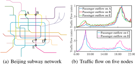
On the other hand, many existing methods only consider the localized spatial correlations. However, we notice that the spatial correlations over different nodes on traffic networks are both local and non-local. It is observed from Figure 1 that the traffic flow of nodes with far distances could have close correlations (see the nodes A, B, and E), while the traffic flow of nodes with short distances could exhibit different characteristics (see the nodes C, D, and E).
According to the above analyses, accurate traffic flow prediction on traffic networks is a very challenging task. To capture the complicated and dynamic spatial-temporal dependencies and solve the problem of traffic flow prediction, we propose a deep Global Spatial-Temporal Network (GSTNet), which consists of several layers of spatial-temporal blocks. Each block contains a multi-resolution temporal module and a global correlated spatial module in sequence. The main contributions of the proposed model are as follows:
- A multi-resolution temporal module with a long receptive field is developed to handle the long-term period-
ical dependencies. In the module, both the short-term neighboring and the long-term periodical dependencies are carefully captured.
- A global correlated spatial module is proposed to learn the spatial correlations on traffic networks. The design of this module is to capture the global correlations between nodes. Thus, the local and non-local spatial correlations on traffic networks can be simultaneously modeled in the same framework.
- The whole model merges together the temporal and spatial modules, which considers the dynamic temporal and the global spatial correlations simultaneously. Extensive experiments verify the effectiveness and superiority of the proposed model.
2 RelatedWork
2.1 Deep Learning on Traffic Prediction
Recently the deep learning based methods for traffic prediction have been largely developed. Specifically, the stacked auto encoder (SAE) [Lv et al., 2015] is first employed to predict traffic states of different nodes. The LSTM network [Hochreiter and Schmidhuber, 1997] and SAE are combined to predict extreme traffic conditions [Yu et al., 2017]. In addition, the convolutional neural networks (CNNs) have also been adopted for predicting the citywide crowd flows [Zhang et al., 2017]. To be specific, the traffic data is transformed into a 32×32 grid image as a heat map, whose pixel value is determined by the traffic flow at each time interval through the grid. Then the CNNs with residual connection [He et al., 2016] are utilized to capture the spatial-temporal traffic patterns. The similar idea is also adopted by the subsequent approaches [Zhou et al., 2018; Yao et al., 2018a; Yao et al., 2018b], some of which are embedded with LSTM network or attention mechanism to further strengthen the model performance. However, directly transforming the traffic data to images distorts and coarsens the spatial relationships between nodes. On the other hand, the graph convolution models can be applied to traffic prediction.
2.2 Deep Learning on Graphs
To make the convolution applicable on graph structured data, the graph convolution is developed from the perspective of spectral domain [Bruna et al., 2013; Henaff et al., 2015]. However, this convolution requires explicit Laplacian eigenvalue decomposition. For this reason, the convolutional kernel is replaced with a multi-order Chebyshev polynomial (ChebNet) [Defferrard et al., 2016], which avoids explicit eigenvalue decomposition. The ChebNet is further modified for semi-supervised graph classification [Kipf and Welling, 2016]. The graph convolution has also been developed directly based on the graph structure, such as the graph convolution network (GCN) [Hechtlinger et al., 2017] and the diffusion convolution [Atwood and Towsley, 2016]. The MoNet (Mixture Model Networks) [Monti et al., 2016] is a general description of the models developed from spatial domain. Besides, the structure-aware convolutional neural networks (SACNNs) [Chang et al., 2018] is proposed for handling the non-Euclidean or graph structured data.
Recently, the graph CNN models have been employed to capture the spatial correlations for traffic prediction. For instance, the Diffusion Convolutional Gated Recurrent Unit (DCGRU) [Li et al., 2018] and LC-RNN [Lv et al., 2018] are developed to capture the localized spatial correlations on traffic networks. The model with multi-graph CNNs [Chai et al., 2018] is proposed to predict the city bike flow. In addition, a fully convolutional spatial-temporal graph neural network [Yu et al., 2018] is developed to extract the features on traffic networks. However, most of the current graph based methods do not notice the non-local spatial correlations between nodes on traffic networks.
3 ProposedModel
3.1 Overview
Notations. The traffic topological network can be represented by a graph G = (V, E), where V stands for the set of nodes, and E describes the accessible routes between nodes. eij ∈ E indicates that there is an edge between two nodes vi and vj. Suppose that there are N nodes and M types of traffic flow data (e.g., inflow and outflow), the m-th type of traffic flow data on node vi at time t is denoted as xi,t,m. The historical traffic flow data with length T obtained along the time axis constitutes a tensor X ∈ RN×T×M .
Problem Statement. The task of prediction problem is to learn a mapping function fθ. The function fθ takes historical traffic data X as well as the graph G as inputs, predicting the traffic flow of all nodes at the next time:
where ˆ X ∈ RN×M denotes the prediction results, and θ stands for the learnable parameters.
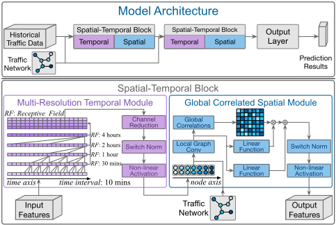
Architecture of Our Designed Network. Figure 2 shows the architecture of the proposed GSTNet, which consists of several layers of spatial-temporal blocks and an output layer. Each spatial-temporal block contains a multi-resolution temporal module and a global correlated spatial module in sequence. The output layer employs an attention mechanism on temporal domain, which automatically selects the relevant historical traffic data. The detailed mechanism of each module is described in the following subsections.
3.2 Multi-Resolution Temporal Module
A multi-resolution temporal module is proposed, which has a long receptive field to capture the long-term periodic dependencies. Thus, both short-term neighboring and longterm periodic dependencies are simultaneously considered. The module is composed by stacking several layers of tensor causal convolution with different dilation rates, which is shown in Figure 2 (left bottom).
Tensor Causal Convolution. The tensor causal convolution is developed to preserve the chronological order of data (the outputs at current time are only related to historical data). The result of causal convolution [Oord et al., 2016] on node vi is as follows:
where yi,t,p is the convolutional result of node vi on the pth channel at time t, d is the dilation rate, and wk,m,p is the element of the convolution kernel. Furthermore, in Eq. (2), all the elements of wk,m,p constitute the convolution kernel W ∈ RKτ×M×P , where Kτ represents the kernel length, and P denotes the number of output channels. In process, zero padding strategy is utilized to keep the temporal length unchanged. Now, applying the same convolution kernel to all nodes yields the following formulation of tensor causal convolution:
where Y ∈ RN×T×P is the output features, and ∗d represents the tensor causal convolution with dilation rate d. Due to the entirely convolutional architecture, the tensor causal convolution has the rapid responses to temporal signals and a flexible receptive field on the temporal axis. The length of the receptive field is Kτ × d, where Kτ is the length of convolution kernel, and d is the dilation rate.
Multi-Resolution Architecture. Multiple layers of tensor causal convolution are stacked, which can not only expand the receptive field on temporal axis, but also obtain the multiresolution outputs. The convolutions of bottom layers are designed to extract short-term neighboring dependencies, and those of higher layers are responsible of learning long-term temporal features. To further expand the receptive field, the dilation rate increases with an exponential speed, i.e., d(l) = 2(l-1) :
where Y l ∈ RN×T×P is the output features of the l-th layer, W(l) ∈ RKτ×M×P is the convolutional kernel, and σ(·) denotes the non-linear activation function. The results Y l of different layers capture the temporal dependencies on different resolutions, which are concatenated to obtain the multiresolution output features:
where Y ∈ RN×T×Q is the output features of the multiresolution temporal module, and Q is the the number of output channels. Furthermore, [Y 1 , Y 2 , · · · , Y L] denotes the operation of tensor concatenation on the channel dimension, and h(·) is the convolution for channel reduction.
3.3 Global Correlated Spatial Module
A global correlated spatial module is developed, which has the capability of extracting the global spatial correlations between nodes on the traffic network. Thus, the local and nonlocal spatial correlations can be simultaneously modeled in the same framework. The proposed module contains a localized graph convolution and a non-local correlated mechanism with the residual connection [He et al., 2016].
Localized Graph Convolution. The graph convolution is first developed from the perspective of Fourier domain [Bruna et al., 2013]. Let x ∈ RN be the signal, and A ∈ RN×N be the adjacent matrix of the graph, the convolution is:
where y ∈ RN is the convolution result, θ is the learnable parameters, and gθ(Λ) = diag(θ) is the filter of a diagonal matrix. Furthermore, in Eq. (6), U ∈ RN×N is the eigenvectors of the normalized Laplacian L = IN -D- 12AD- 12 = UΛUT, where Λ ∈ RN×N is the corresponding eigenvalues, IN is the identity matrix with N dimension, and D is the diagonal degree matrix with Di,i = ∑j Ai,j . Since L is positive semidefinite, U is an orthogonal matrix. In Eq. (6), the signal x is first transformed to the Fourier domain ˆx = UTx. A diagonal matrix gθ(Λ) is used as the filter to adjust the amplitude of the transformed signal ˆx. Finally, the modulated signal is transformed back to the spatial domain. Although the convolution of Eq. (6) is theoretically guaranteed, it suffers from the requirements of explicit Laplacian eigenvalue decomposition and the non-localized filters on spatial domain. For these reasons, the convolution kernel is replaced with the Chebyshev polynomial [Defferrard et al., 2016]:
where y ∈ RN is the convolutional result, θk is the learnable parameter, and Tk(˜L) is the k-th order Chebyshev polynomial, with the rescaled Laplacian ˜L = 2L/λmax - IN. Here λmax is the maximal value among the eigenvalues of L, In Eq. (7), ¯xk can be recursively computed by ¯xk = 2˜L¯xk-1 - ¯xk-2, with ¯x0 = x, and ¯x1 = ˜Lx. It is worth pointing out that ¯xk only contains the features of the k-th order adjacent nodes at most. Thus, the convolution is strictly localized on spatial domain, with a receptive field of length K - 1: y = θ ∗G x, where θ = [θ0, θ1, · · · , θK-1]T ∈ RK is the convolution kernel. Now, the localized graph convolution can be applied to extract the local spatial correlations between nodes on the traffic network. For node vi, the extracted features at the t-th historical time is denoted as a vector yi,t ∈ RQ, where Q is the number of channels on each node. The features of all nodes constitute a feature matrix Yt = [y1,t, y2,t, · · · , yN,t]T ∈ RN×Q, and the result of graph convolution is:
where ˆYt = [ˆ y1,t, ˆ y2,t, · · · , ˆ yN,t]T ∈ RN×D represents the output features, and ˆ yi,t ∈ RD denotes the localized spatial features on node vi at time t. Furthermore, in Eq. (8), Θ ∈ RKs×Q×D is the convolution kernel, where Ks is the kernel length, and D is the number of output channels.
Global Spatial Correlations. The non-local correlated mechanism is constructed to extract the non-local spatial correlations between nodes, as shown in Figure 2 (right bottom):
where zi,t ∈ RF is the output features on node vi at time t, F is the number of output channels, and φ(·, ·) is a bivariate function. Furthermore, si,j is the global topological weight (si,j = β ≥ 1 if ei,j ∈ E, otherwise si,j = 1), and g(·) transforms the features on node vj. In Eq. (9), φ measures the global correlations between nodes, and "+ ˆ yi,tWr" denotes the residual connection with the localized features, where Wr ∈ RD×F is the learnable parameters. The addition of topological weight si,j makes the non-local correlated mechanism not only consider the dynamic correlations between nodes, but also the static topological structure of the traffic network. For practicality, g(ˆ yj,t) = ˆ yj,tWg is the linear function and φ is the embedded Gaussian kernel φ(x, y) = exp(xTWφy) and the learnable dot product φ(x, y) = xTWφy, respectively, where Wg ∈ RD×F and Wφ ∈ RD×D are the learnable parameters. The output features zi,t of all nodes at all historical times can be efficiently computed in parallel, and composed to obtain the output tensor:
where Z ∈ RN×T×F is the outputs of the spatial module.
3.4 Model Summarization
To capture the dynamic temporal and the global spatial correlations simultaneously, the spatial-temporal block is constructed. Each block contains a multi-resolution temporal module and a global correlated spatial module in sequence, which is shown in Figure 2 (top). Several layers of the spatialtemporal blocks are stacked, followed by an output layer to predict the future traffic states. The output layer employs an attention module [Vaswani et al., 2017] on temporal axis to adaptively select the most relevant historical traffic data:
where ˆ X is the prediction results, Zt ∈ RN×F is the spatialtemporal features at time t, and Xt+1 ∈ RN×M is the historical traffic data at time t + 1. Furthermore, Wo ∈ RM×M is the learnable parameters, and ψ(·, ·) is the Frobenius inner product of two matrices. In Eq. (11), ψ(ZT ,Zt) measures the relevances of the spatial-temporal features between historical times (Zt) and the current time (ZT ), which are then exploited to map the historical traffic data to the traffic states at the next time. Finally, the MSE loss function is adopted to train the model:
where ˜ X ∈ RN×M is the ground truth at the next time T +1. Now we summarize our GSTNet method as follows: (1) Each spatial-temporal block can not only capture the short term neighboring and the long term periodical temporal dependencies, but also take the global spatial correlations into consideration, with few learning parameters. (2) Several layers of stacked spatial-temporal blocks constitute the framework for handling structured data with chronological order. (3) The whole model can be efficiently trained through highly parallelized mechanisms and affordable computing resources.
4 Experiments
4.1 Datasets
The proposed method is verified on three real-world traffic datasets. The first two datasets are the transaction records of Beijing Subway and Bus System, and the third dataset is the taxi GPS trajectories in Beijing. Detailed information of the datasets is reported in Table 1.
| Properties | Datasets | ||
|---|---|---|---|
| Subway | Bus | Taxi | |
| # Nodes | 278 | 24 | 198 |
| Time interval | 10 mins | 1 hour | 20 mins |
| Time span | 2016/6/1 - | 2016/6/29 | 2015/11/1 - 2016/5/31 |
| Daily range | 6:00-22:00 | ||
| Models | Subway Dataset | Bus Dataset | Taxi Dataset | |||
|---|---|---|---|---|---|---|
| MAE | MAPE (%) | MAE | MAPE (%) | MAE | MAPE (%) | |
| HA | 49.76 | 30.38 | 26.18 | 38.27 | 52.21 | 33.45 |
| SAE | 26.52 ± 0.86 | 25.60 ± 1.14 | 12.34 ± 0.94 | 21.56 ± 1.71 | 35.07 ± 0.44 | 24.26 ± 0.32 |
| LSTM | 26.93 ± 0.17 | 26.53 ± 0.27 | 17.34 ± 1.38 | 24.76 ± 1.36 | 35.75 ± 0.12 | 25.17 ± 0.19 |
| ChebNet | 28.19 ± 2.40 | 24.89 ± 2.11 | 13.57 ± 1.67 | 22.21 ± 2.14 | 37.08 ± 3.08 | 27.52 ± 2.71 |
| GCGRU-GCN | 26.64 ± 0.15 | 26.02 ± 0.27 | 18.60 ± 0.60 | 26.15 ± 1.04 | 35.53 ± 0.29 | 24.92 ± 0.33 |
| STGCN-Action | 26.90 ± 0.61 | 22.72 ± 0.72 | 11.81 ± 0.70 | 18.93 ± 0.71 | 38.92 ± 1.28 | 26.31 ± 1.15 |
| GSTNet (Product) | 24.30 ± 1.12 | 21.02 ± 0.78 | 11.11 ± 0.24 | 18.15 ± 0.64 | 31.72 ± 0.26 | 21.67 ± 0.24 |
| GSTNet (Gaussian) | 23.19 ± 0.43 | 19.78 ± 0.29 | 11.04 ± 0.34 | 18.26 ± 0.34 | 32.18 ± 0.49 | 21.92 ± 0.47 |
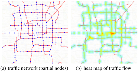
Subway Transactions Dataset. The Beijing subway transaction records include the entering and exiting nodes as well as the entering and exiting timestamps of each transaction. It can be easy to infer the passenger flow of all nodes in all time intervals. For most of the subway lines are closed at night, only the records from 6:00 to 22:00 are considered. Figure 3 shows the traffic network (partial nodes) and the heat map of the passenger outflow at one time interval on the network.
Bus Transactions Dataset. The basic characteristics of the Bus Transactions Dataset are the same as those of the Subway Dataset. There are totally more than 4,500 bus stops and the computing costs of all stops can be expensive, and thus the bus Line One and the nodes on this line are taken into consideration (see Table 1 for more details).
Taxi Trajectories Dataset. The third dataset contains the trajectories of all taxis (more than 30,000 taxis) in Beijing. 198 major intersections are chosen as nodes to compute the traffic flow through these nodes in each day (see Table 1 for more details).
4.2 Experimental Settings
All the models utilize two days of historical traffic data and predict the traffic flow at the next one time interval.
Network Structure and Learning Strategy. The model contains two layers of spatial-temporal blocks. The temporal module consists of three convolution layers. The length of convolution kernel is three in each layer, and the output
(b) Prediction error during one week
Figure 4: Detailed prediction results of Subway Dataset.
channels is 8. The 24 output channels are then reduced to 8 channels. The hidden channels and output channels in spatial module is set to 8. The length of graph convolution kernel is three. The embedded Gaussian kernel is the default option. The hyperparameter β is set to β = 2. LeaklyReLU is selected as the non-linear activation function. The normalization method is chosen as the Switchable Normalization [Luo et al., 2018]. The optimizer is the Adam algorithm [Kingma and Ba, 2014] and the learning rate is set to α = 1e-3 .
Compared Algorithms. Several traditional shallow models and competitive deep learning models are selected as the compared algorithms: (1) HA: Historical Average. (2) LSTM: Long Short Term Memory. (3) SAE [Lv et al., 2015]: Stacked Auto Encoder. (4) ChebNet [Defferrard et al., 2016]: Graph CNN with Chebyshev polynomial kernel. (5) GCRNN-GCN [Li et al., 2018]: Graph Convolution Recurrent Neural Network with GCN [Hechtlinger et al., 2017] kernel. (6) STGCN-Action [Yan et al., 2018]:
Spatial-temporal graph convolutional networks for skeletonbased human action recognition, where the last layer is modified for traffic prediction.
Evaluation Metrics. Two most-widely adopted metrics, MAE (Mean Absolute Error), and MAPE (Mean Absolute Percentage Error), are employed to measure the performance of different methods.
4.3 Experimental Results
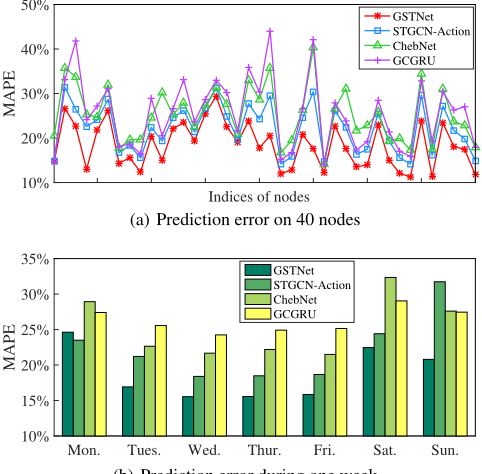
Model Comparsion. Table 2 reports the experimental results on the three datasets of Beijing Subway, Bus, and Taxi Datasets. All the uncertainties are computed by re-training the models with random seeds and modified by a Student's t-distribution with a confidence probability of P = 0.9. The proposed GSTNet achieves best predicting accuracy and satisfying uncertainties on all metrics and all datasets. As the RNN based models do not effectively exploit the spatial correlations, and the receptive field on temporal axis is limited, the prediction accuracy is worse than the proposed model (see the results of LSTM and GCGRU). Figure 4(a) illustrates the average MAPE error on each node of the Subway Dataset. Similar conclusions can be extended to other two datasets. Only the results of 40 nodes are displayed for clarity. It is observed that the proposed GSTNet outperforms other methods on different nodes, demonstrating that the proposed model is advanced on spatial domain. Figure 4(b) shows the average performance of different models during a week. In the figure, except for the slightly higher error on Monday, the proposed GSTNet achieves best results in all other days, illustrating that the GSTNet is also excellent on temporal dimension.
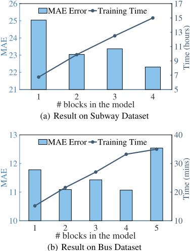
Number of Spatial-Temporal Blocks in the Model. To determine the appropriate number of spatial-temporal blocks in the proposed model, models with different number of blocks are compared. Figure 5 illustrates the experimental results on Subway and Bus Datasets. It is observed that more blocks lead to the increase of the training time, but the improvement of model performance is limited. In addition, too many blocks could cause over-fitting. Therefore, the model with two spatial-temporal blocks is appropriate, with satisfying results and affordable training time.
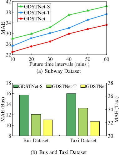
Evaluation of Spatial and Temporal Modelings. To verify the effectiveness of the spatial and temporal modelings, two variants are compared with the proposed GSTNet:
- GSTNet-S (patial): the same structure as the GSTNet except that there are only spatial modules.
- GSTNet-T (emporal): the same structure as the GSTNet except that there are only temporal modules.
Figure 6(a) shows the MAE error of different predicting future time steps on the Subway Dataset and Figure 6(b) illustrates the results on the other two datasets. It is observed that the performance improvement brought by the combination of temporal and spatial modelings is superior to that of adopting one of them, with different datasets and different predicting future time steps. Such a result demonstrates the effectiveness of the proposed temporal and spatial modules.
Evaluation of Non-local Properties. To evaluate the nonlocal properties on traffic networks, the proposed GSTNet is compared with two variant models:
- GSTNet-I (dentity): No topological structure information is considered, i.e., the graph G is replaced by an identity matrix I.
- GSTNet-L (ocal): Only the local correlations are considered in the spatial modules.
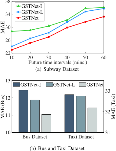
Figure 7 gives the prediction results on the three datasets. In the figure, the proposed model with global spatial correlations performs best results, compared with other two variants. It is also observed from Figure 7(a) that the local spatial correlations could be weak in long-term prediction tasks (see the results of GSTNet-I and GSTNet-L in 50 and 60 mins), while the global spatial correlations could be more essential to longterm prediction.
Time Comparison. Table 3 gives the results of time comparison between different models on the Subway Dataset. Similar conclusions can be extended to other two datasets. For a fair comparison, the training time is computed on one epoch, and the test time is operated on all of the test samples. All the models are compared under the same computing resources. It is observed from Table 3 that the running time of the proposed model achieves a compromise between the RNN based models (GCGRU and LSTM) and the graph convolution models (ChebNet and STGCN), and meanwhile obtains the best prediction accuracy.
Results onPeMSDataset. To further verify the generalization of the proposed model, different methods are also compared on a public dataset: the PeMS-BAY Dataset [Li et al., 2018] for traffic speed prediction. The experimental results are reported on Table 4. From the results, it is observed that our model achieves the best accuracy. This demonstrates a good generalization of the proposed model.
5 Conclusion
This paper proposes a novel deep learning model for predicting traffic flow on traffic networks, integrating a multiresolution temporal module and a global correlated spatial module. Experiments on the real-world datasets verify the effectiveness and superiority of the proposed method on two kinds of traffic networks (public transportation network and road network) and three types of datasets (subway, bus and taxi). In the future, we will extend our framework for addressing multi-step and long-term prediction.
| Models | Subway Dataset | |
|---|---|---|
| Training (mins) | Test (mins) | |
| SAE | 0.20 | 0.03 |
| STGCN-Action | 0.10 | 0.03 |
| ChebNet | 0.11 | 0.03 |
| GSTNet | 1.42 | 0.22 |
| GCGRU-GCN | 3.84 | 1.28 |
| LSTM | 6.76 | 1.64 |
| Models | PeMS-BAY Dataset | |
|---|---|---|
| MAE | MAPE (%) | |
| HA | 4.83 | 9.91 |
| SAE | 3.34 | 8.41 |
| LSTM | 2.88 | 6.96 |
| ChebNet | 2.61 | 4.95 |
| GCGRU-GCN | 3.16 | 7.75 |
| STGCN-Action | 3.45 | 8.18 |
| GSTNet | 1.94 | 3.53 |
Acknowledgments
This work was supported by the National Natural Science Foundation of China under Grants 91646207, and 61773377, and the Beijing Natural Science Foundation under Grant L172053.
@inproceedings{ijcai2019p317,
  title     = {GSTNet: Global Spatial-Temporal Network for Traffic Flow Prediction},
  author    = {Fang, Shen and Zhang, Qi and Meng, Gaofeng and Xiang, Shiming and Pan, Chunhong},
  booktitle = {Proceedings of the Twenty-Eighth International Joint Conference on
               Artificial Intelligence, {IJCAI-19}},
  publisher = {International Joint Conferences on Artificial Intelligence Organization},
  editor    = {Sarit Kraus},
  pages     = {2286--2293},
  year      = {2019},
  month     = {8},
  note      = {Main track},
  doi       = {10.24963/ijcai.2019/317},
  url       = {https://doi.org/10.24963/ijcai.2019/317},
}
TY - CPAPER TI - GSTNet: Global Spatial-Temporal Network for Traffic Flow Prediction AU - Fang, Shen AU - Zhang, Qi AU - Meng, Gaofeng AU - Xiang, Shiming AU - Pan, Chunhong T2 - Proceedings of the Twenty-Eighth International Joint Conference on Artificial Intelligence, IJCAI-19 PB - International Joint Conferences on Artificial Intelligence Organization PY - 2019 SP - 2286 EP - 2293 DO - 10.24963/ijcai.2019/317 UR - https://doi.org/10.24963/ijcai.2019/317 ER -Copied
Machine-readable versions of this paper, for tools and AI agents:





