
Jointly Learning Network Connections and Link Weights in Spiking Neural Networks
Proceedings of the Twenty-Seventh International Joint Conference on Artificial Intelligence. Main track. Pages 1597-1603.
https://doi.org/10.24963/ijcai.2018/221
Keywords
- Humans and AI: Cognitive Systems
- Machine Learning: Neural Networks
- Humans and AI: Brain Sciences
- Humans and AI: Cognitive Modeling
- Machine Learning: Machine Learning
Abstract
Spiking neural networks (SNNs) are considered to be biologically plausible and power-efficient on neuromorphic hardware. However, unlike the brain mechanisms, most existing SNN algorithms have fixed network topologies and connection relationships. This paper proposes a method to jointly learn network connections and link weights simultaneously. The connection structures are optimized by the spike-timing-dependent plasticity (STDP) rule with timing information, and the link weights are optimized by a supervised algorithm. The connection structures and the weights are learned alternately until a termination condition is satisfied. Experiments are carried out using four benchmark datasets. Our approach outperforms classical learning methods such as STDP, Tempotron, SpikeProp, and a state-of-the-art supervised algorithm. In addition, the learned structures effectively reduce the number of connections by about 24%, thus facilitate the computational efficiency of the network.
- [Bi and Poo, 2001] Guoqiang Bi and Muming Poo. Synaptic modification by correlated activity: Hebb's postulate re- visited. Annual Review of Neuroscience, 24(1):139-166, March 2001.
- [Bohte et al., 2002] Sander M. Bohte, Joost N. Kok, and Han La Poutré. Error-backpropagation in temporally encoded networks of spiking neurons. Neurocomputing, 48(1):17- 37, October 2002.
- [Dheeru and Karra Taniskidou, 2017] Dua Dheeru and Efi Karra Taniskidou. UCI machine learning repository, 2017.
- [Diehl and Cook, 2015] Peter U. Diehl and Matthew Cook. Unsupervised learning of digit recognition using Spike- Timing-Dependent Plasticity. Frontiers in Computational Neuroscience, 9:99, August 2015.
- [Eurich and Wilke, 2000] C Eurich and S Wilke. Multidi- mensional encoding strategy of spiking neurons. Neural Computation, 12(7):1519-1529, July 2000.
- [Filip, 2005] Ponulak Filip. ReSuMe new supervised learn- ing method for Spiking Neural Networks. Institute of Con- trol and Information Engineering, Poznan University of Technology., 2005.
- [Gerstner and Kistler, 2002] Wulfram Gerstner and Werner M. Kistler. Spiking neuron models: single neurons, populations, plasticity. Cambridge University Press, Cambridge, 2002.
- [Ghosh-Dastidar and Adeli, 2009] S. Ghosh-Dastidar and H. Adeli. Spiking neural networks. International Jour- nal of Neural Systems, 19(04):295-308, August 2009.
- [Gütig and Sompolinsky, 2006] Robert Gütig and Haim Sompolinsky. The tempotron: a neuron that learns spike timing-based decisions. Nature Neuroscience, 9(3):420- 428, March 2006.
- [Hebb, 1949] D. O. Hebb. In the organization of behavior: a neuropsychological theory. John Wiley , Chapman and Hall, 1949.
- [Hinton and Salakhutdinov, 2006] G. E. Hinton and R. R. Salakhutdinov. Reducing the dimensionality of data with Neural Networks. Science, 313(5786):504-507, July 2006.
- [Hodgkin and Huxley, 1952] A. L. Hodgkin and A. F. Hux- ley. A quantitative description of membrane current and its application to conduction and excitation in nerve. The Journal of Physiology, 117(4):500-544, August 1952.
- [Maass, 1997] Wolfgang Maass. Networks of spiking neu- rons: The third generation of neural network models. Neu- ral Networks, 10(9):1659-1671, December 1997.
- [Masquelier et al., 2009] Timothée Masquelier, Rudy Guy- onneau, and Simon J. Thorpe. Competitive STDP-based spike pattern learning. Neural computation, 21(5):1259- 1276, May 2009.
- [Ranhel, 2012] J. Ranhel. Neural assembly computing. IEEE Transactions on Neural Networks and Learning Systems, 23(6):916-927, June 2012.
- [Shatz, 1992] C. J. Shatz. The developing brain. Scientific American, 267(3):60-67, September 1992.
- [Tsukada and Pan, 2005] M. Tsukada and X. Pan. The spatiotemporal learning rule and its efficiency in sepa- rating spatiotemporal patterns. Biological Cybernetics, 92(2):139-146, February 2005.
- [Xie et al., 2017] X. Xie, H. Qu, Z. Yi, and J. Kurths. Effi- cient training of supervised Spiking Neural Network via accurate synaptic-efficiency adjustment method. IEEE Transactions on Neural Networks and Learning Systems, 28(6):1411-1424, June 2017.
- [Yu et al., 2013a] Q. Yu, H. Tang, K.C. Tan, and H. Li. Precise-Spike-Driven synaptic plasticity: learning Hetero- Association of spatiotemporal spike patterns. PLOS ONE, 8(11):e78318, November 2013.
- [Yu et al., 2013b] Q. Yu, H. Tang, K.C. Tan, and H. Li. Rapid feedforward computation by temporal encoding and learning with spiking neurons. IEEE Transactions on Neu- ral Networks and Learning Systems, 24(10):1539-1552, October 2013.
References were extracted automatically from the PDF and may contain errors.
Full text extracted automatically from the PDF; figures, tables and equations may differ. The PDF is the version of record.
1 Introduction
Artificial neural networks (ANNs) have obtained great success in the computer vision and pattern recognition fields in recent years. Although ANNs are inspired by brain, most studies only imitate layer-like brain structures roughly [Hinton and Salakhutdinov, 2006]. Spiking neural networks (SNNs), known as the third generation of artificial neural network, work in the manner of spiking neurons in brain, thus are more biologically plausible and have potential to approach the intelligence of brain [Tsukada and Pan, 2005] [GhoshDastidar and Adeli, 2009] [Maass, 1997]. However, existing SNN algorithms usually have fixed network topologies and connection relationships. According to the Hebbian theory [Hebb, 1949], only a few cells would strongly connect together when brain transfers information, e.g. the persistently co-active cells. Therefore, how to build a spiking neural network with both optimal connection and link weights is an important problem.
∗Corresponding author: gpan@zju.edu.cn
Much effort has been made on structure design and learning of SNN. Various spiking neuron models, such as the leaky integrate-and-fire (LIF) model [Gerstner and Kistler, 2002] and the Hodgkin-Huxley type model [Hodgkin and Huxley, 1952], have been proven to be capable of encoding temporal information in synapses between neurons. To improve the learning capacity in SNN, different approaches including unsupervised rules and supervised algorithms were proposed.
- Unsupervised learning methods. The unsupervised approaches are mostly biomimetic methods inspired by the mechanism in biological neurons. The Hebbian theory, which is often summarized as 'Cells that fire together wire together' [Shatz, 1992], is considered to be the foundation of connection learning in biological neurons. According to the Hebbian theory, the spiketiming-dependent plasticity (STDP) rule has been proposed which exploits the timing and the emitting order of the spikes [Bi and Poo, 2001]. The STDP algorithm strengthens a weight when the presynaptic neuron emits spikes preceding the postsynaptic one, and weakens it when the order is reversed. Recently, lots of STDPbased approaches are proposed with promising results [Diehl and Cook, 2015] [Masquelier et al., 2009]. Despite the effectiveness of the unsupervised methods, the convergence of these approaches can not be guaranteed due to the difficulty in setting appropriate parameters.
- Supervised learning methods. Some supervised rules were proposed in order to accelerate the learning progress. With the help of instructor signals, supervised algorithms can potentially improve the learning speed. Classical supervised learning algorithms are mostly based on gradient descent methods. SpikeProp [Bohte et al., 2002] is one of the representative learning algorithms to process spatiotemporal information in SNN. The Tempotron rule [G¨utig and Sompolinsky, 2006] then extends the ability of SNN to binary classification tasks. Another type of supervised training approach uses learning windows. Unlike the gradient descent methods that minimize the cost functions, these methods such as the remote supervised learning method (ReSuMe) [Filip, 2005] and the precisespike-driven (PSD) [Yu et al., 2013a] are motivated by the Widrow-Hoff rule, and use the Hebbian and anti-
Hebbian learning windows to drive training. The training window-based algorithms are commonly more efficient than methods with gradient descent rules.
Although various learning methods have been proposed, joint optimization of SNN connections and link weights has not been well addressed. In this study, we propose a method to jointly learn network connections and link weights simultaneously in SNNs. To enable structure learning, we propose a spiking neuron with connection gate (SNN-CG) to control whether a connection should be established. A connection weight is effective only if the gate is open. In SNN-CG, the connection gates are learned based on the Hebbian theory and the STDP rule. The link weights are updated using a supervised algorithm. The structure learning and weight updating work alternately until a termination condition is satisfied. Experiments are conducted using four benchmark datasets. Our approach outperforms classical learning methods such as STDP, Tempotron, SpikeProp, and a state-of-the-art work with better accuracies in classification tasks. Besides, the learned network structure effectively reduces the number of connections in a data-driven way, which further facilitate the computational efficiency of the network.
2 Method
In this section, we present the SNN-CG algorithm in details. We first introduce the formulations of the spiking neural networks with connection gates. Then we elaborate the STDP rule-based connection learning and supervised link weight updating algorithms respectively. Finally, we present the iterative training scheme to jointly learn both connection structures and the corresponding weights.
2.1 SNNwith Connection Gates
In order to enable structural learning of connections between neurons, we assemble connection gates to the SNN model. We start from the classical leaky integrate-and-fire (LIF) neuron model and then describe the model with connection gates.
LIF neuron model. Given an LIF neuron j, suppose there are N presynaptic afferents contributing to it. Neuron j is driven by exponential decaying synaptic currents generated by its N presynaptic neurons. Then the subthreshold membrane voltage of neuron j is a weighted sum of postsynaptic potentials (PSPs) contributed by all incoming spikes:
where Wij is the synaptic efficacy between postsynaptic neuron j and presynaptic afferent i, ti and Vrest denote the firing time of presynaptic afferent i, and the rest potential of postsynaptic neuron j, respectively. A normalized PSP kernel K vanishing for ti > t is as follows:
where V0 is used to normalize the maximum of kernel to be 1.0, which ensures unitary PSP amplitudes to be given by synaptic efficacies Wij . The parameters τm and τs denote the decay time constants of membrane integration and synaptic currents, respectively. The postsynaptic neuron j fires a spike once its voltage Vj crosses the firing threshold Vthr. That is, neuron j generates an output spike at that time. Since we only consider the situation that postsynaptic neuron is fired only once in this paper, the voltages of that fired neuron smoothly decline to Vrest by shutting down all the following incoming spikes.
Connection gates. Based on LIF, we enable structural learning by using connection gates in the links between neurons, called spiking neural network with connection gates (SNN-CG). The connection gates control whether two neurons are linked with each other. With the connection gate Gij between neurons i and j, (1) can be rewritten as follows:
With a proper connection adjusting rule, the SNN-CG model establishes connections between neurons only if they are related. Therefore, the neurons become more sensitive to related neurons, and thus are able to transmit information more effectively and robustly than fully connected networks.
Gate functions. The connection gates in SNN-CG model can be implemented using different functions. We apply the sigmoid function as the gate function in this work:
where bij is the connecting coefficient between neuron i and neuron j. A higher bij indicates stronger connections.
2.2 Connection Learning
In biological systems, the links between neurons are adjusted using the timing information in spikes. According to the Hebbian theory, repeatedly and persistently co-active cells would increase connective synaptic efficacy among populations of interconnected neurons [Hebb, 1949].
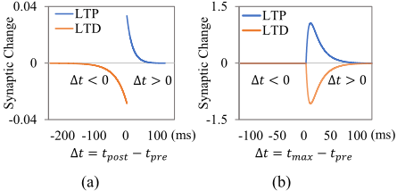
Motivated by the biological mechanism, we adopt the STDP rule to learn the connections in SNN neurons. The STDP rule provides powerful guidance for establishing or eliminating the connections between neurons by considering both the timing and the order of the spikes. The plasticity in STDP depends on the intervals between presynaptic and postsynaptic spikes. As illustrated in Fig. 1 (a), a connection is strengthened (long-term potentiation, LTP) when the presynaptic neuron emits spikes preceding the postsynaptic one and weakened (long-term depression, LTD) when the order is reversed. The STDP rule used is as follows:
where the parameters τ + and τ - determine the ranges of pre-to-postsynaptic interspike intervals on which synaptic strengthening and weakening occur. A+ and A- refer to the maximum amounts of synaptic modification for LTP and LTD, respectively. The ratio between the A+ and A- balances the magnitudes of strengthening and weakening of the connections in STDP.
According to the STDP rule, the connection gate can be updated based on W stdp ij :
where λc is the learning rate for connections, and bij is the connecting coefficient between neuron i and neuron j. With the STDP-based connection learning, the connections between related neurons are strengthened toward one and the connections between unrelated neurons decay to zero.
2.3 Weight Learning
The link weights in SNN can be learned with general supervised learning methods suitable for temporal coding. In this study, we employ Tempotron rule due to its good ability for classification.
In binary classification, the input patterns to the neurons belong to one of two types of ⊕ and ⊖. When a ⊕ is presented to the neuron, it fires a spike, and when a ⊖ appears, the neuron does not fire. Tempotron rule learns the synaptic weights of Wij with gradient descent to minimize the error signals:
where tmax is the time point that the neuron reaches its maximum voltage, and Vthr is the threshold for neurons to fire a spike. The gradients of parameter Wij are computed follows:
where λw is the weight learning rate. ⊕ error means the error that the neuron should emit but it does not, and ⊖ error is the error that the neuron should not emit but it does. The learning window of the Tempotron rule is illustrated in Fig 1 (b). According to the kernel shape, the spikes near tmax change more than those far away from it.
2.4 Iterative Training
To jointly learn the connections and the link weights, we propose an iterative learning scheme. In the connection learning stage, the weights of the links are fixed and the connection
Algorithm 1 Iterative Training Algorithm of SNN-CG.
Initialization:
- 1: Im =M, In = N.
- 2: W ∈ [-0.01, 0.01].
- 3: Wstdp = 0, G= 0.5 × I.
Output: W and G.
- 4: procedure ITERATIVE TRAINING PROCESS(Wstdp,W)
- 5: while k < Niteration do
- 6: W ←W-update(G, Im)
- 7: G←G-update(Wstdp, In)
- 8: end while
- 9: return G, W ▷ Iterative training
- 10: end procedure
- 1: procedure G-UPDATE(Wstdp, In)
- 2: while q < In do
- 3: ∀j ∀i,W stdp ij ←A±exp( tj-ti τ ± )
- 4: ∀j ∀i, bij ← λcW stdp ij
- 5: ∀j ∀i,Gij ← 1 1+exp(-bij )
- 6: end while
- 7: return G ▷ Connection learning
- 8: end procedure
- 1: procedure W-UPDATE(G, Im)
- 2: while p < Im do
- 3: ∀j ∀i, Wij ← ±λw ∑ti<tmax Gij K(tmax - ti)
- 4: end while
- 5:
- return W ▷Weight learning
- 6: end procedure
strengths are tuned by the STDP rule. In the weight learning stage, the connections are fixed and the weights are updated. The connection learning and the weight learning stages are conducted alternately until a termination condition is satisfied. The details of the iterative training process are presented in Algorithm 1. The key parameters in the iterative training algorithm are M and N, which indicate how many epochs to train in the weight learning stage and connection learning stage respectively.
2.5 Network Architectures
The network includes an encoding layer and a decoding layer. The encoding layer converts the real-valued features into spike trains. The decoding layer determines the classification results using the population decoding method [Yu et al., 2013b].
Encoding layer. The continuous feature values are encoded into spike trains using the Gaussian receptive field method [Bohte et al., 2002] [Eurich and Wilke, 2000]. Suppose a feature value x is in range [xmin, xmax], and it is encoded by different Nencode Gaussian receptive fields. The center and width of the kth Gaussian kernel are defined as µk = xmin + (2k - 3)/2(xmax - xmin)/(Nencode - 2), and σk = 1/1.5(xmax - xmin)/(Nencode - 2), respectively. With the Gaussian kernels, a feature value x is encoded to spike arrays of Nencode dimensions. Because the Tempotron model only permits postsynaptic neuron to fire only once, there are Nencode neurons for each attribute. With the encoding method, the higher activated neurons fire earlier, and vice versa. Suppose there are a total of Nfeature features. Then there are Nencode ×Nfeature neurons in the input layer of the network.
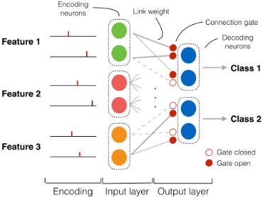
Decoding layer. The binary outputs of networks predict the class labels by population decoding [Yu et al., 2013b], according to the biological mechanisms in neurons [Ranhel, 2012]. For classification, each class is represented by a group of Ndecode neurons. The decisions are made by majority voting, and the incoming samples are classified into the class with maximum numbers of firing neurons. Suppose there are Nclass of classes. The total number of output neurons is Ndecode ×Nclass. The architecture of the SNN-CG method is illustrated in Fig. 2.
Network. We use a single-layer SNN model. The neurons of the encoding layer are fully connected with neurons in the decoding layer by gated links. The connections and the link weights can be jointly adjusted in training. Fig. 2 shows a simple example of the network with three features and two classes.
3 Experiments
In this section, experiments are carried out to evaluate the performance of our method. Firstly, we give the detail of the evaluation datasets and settings. Then we assess the influence of the model settings in SNN-CG, including parameters in connection learning and iterative training. Finally, we compare our approach with existing methods to demonstrate the strength of the SNN-CG model.
3.1 Datasets
Four datasets are used in our experiments. The datasets are selected from the OpenML and the UCI repositories [Dheeru and Karra Taniskidou, 2017]. The detail of the datasets is as follows.
- Iris. A benchmark dataset for plant classification. It contains three types of iris plants with four-dimensional features. There are a total of 150 instances in the dataset.
- Breast Cancer. A binary classification dataset for breast
cancer recognition. It contains 295 samples, and each sample has nine features.
- Liver Disorder. A binary classification dataset for liver disease detection. There are a total of 345 samples in the dataset. For each sample, the dimension of feature is six.
- Pima Indians Diabetes. The dataset includes 500 instances of two classes. The instances are described by eight-dimensional features.
3.2 Settings
Here we give the detail of the configurations of our model, including the model settings and the parameters in training.
For the network architecture, a one-layer SNN-CG model is adopted. For the LIF neuron model, the parameters are set as follows: Vthr = 1.0mV , Vrest = 0mV , V0 = 0.4725mV , τm = 4τs = 15ms. For each feature, the encoding neuron number Nencode is set to 12, and the number of decoding neurons Nencode for each class is set to 8. In the initialization, the connection coefficients b are set to 0.5 ∗ I for the connections gates. The link weights in the network are randomly initialized in the range of [-0.01, 0.01].
For connection learning, the time constants are set to τ + = 16.8ms and τ - = 33.7ms in accordance to the observed measurements experimentally [Bi and Poo, 2001]. The learning rate of connection gates is λc = 1.0.
The performance is evaluated by the classification accuracy. For each dataset, we split the data to ten parts randomly. The experimental result is the average accuracy of the ten parts with cross-validation.
3.3 Influence of the Parameters
In this section, we assess the influence of the parameters in the SNN-CG model. Firstly, we compare the models with different parameters in connection learning. Then we evaluate the parameters in iterative training of connection learning and weight updating.
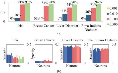
Connection learning. Here we test the influence of the learning parameters in STDP-based connection training. We tune the synaptic modification magnitude of A+ and A- in (5) to change the balance between strengthening and weakening of the connections. In the STDP rule, the ratio between the two parameters is considered to be important. In the experiment, we set the A+ = 0.0156 and A- = 0.02656. Then we tune the ratio between them by multiplying the value of A- with a coefficient C in the range of 0.001 to 0.5. The criteria of performance are the classification accuracy and the connection sparsity. The connection sparsity is computed as the proportion of disconnected links. The links with connection weights lower than 1e-8 are considered to be disconnected. In training, for each iteration, we use M = 100 epochs for weight learning and N = 10 epochs for connection learning.
Fig. 3 illustrates the connection sparsity under different settings. As shown in Fig. 3 (a), the heights of the bars indicate the proportions of disconnected links. With a larger parameter C, the connections in the networks are more sparse. For the Iris dataset, when C = 0.001, the network is almost fully connected. When we tune C to 0.5, 97% of the connections are disconnected. It is reasonable because with a larger C, the STDP rule is prone to weaken a connection. We also investigate the distribution of the connection sparsity over the decoding neurons. Fig. 3 (b) illustrates the sparsity of the decoding neurons with C = 0.01. For the Liver Disorder and Pima Indians Diabetes datasets, the sparsity of the neurons is similar, while for the datasets of Iris and Breast Cancer, the neurons representing different classes exhibit different sparsity.
| Dataset | C=0.001 | C=0.01 | C=0.1 | C=0.5 |
|---|---|---|---|---|
| Iris | 0.9467 | 0.9667 | 0.9133 | 0.7600 |
| Breast Cancer | 0.9542 | 0.9571 | 0.9270 | 0.8470 |
| Liver Disorder | 0.6162 | 0.6214 | 0.6210 | 0.5429 |
| Pima Indians Diabetes | 0.7238 | 0.7304 | 0.6966 | 0.6353 |
The classification performance under different parameters C is illustrated in Table. 1. Overall, the best classification accuracies are obtained when C = 0.01. The accuracies are 96.67%, 95.71%, 62.14%, and 73.04% for the four datasets, respectively. Combining the results in Fig. 3 (b), when we tune C from 0.001 to 0.01, the performance increases despite the amount of connection is reduced. Since the STDP-based connection learning rule removes the unuseful connections, the neurons are more focused on the informative neurons. Therefore, the network becomes more robust than the fully connected structures. However, when we continue increasing the value of C to 0.1, the performance of the SNN-CG model decreases. This is because, with too many connections weakened, the useful connections can be lost, thus lower performance is obtained.
It is interesting to see that, the SNN-CG model is able to achieve good performance even with highly sparse connections. When the parameter C is set to 0.1, the proportion of disconnected links changes from 73% to 91% for the datasets. However, the classification performance only decreases by less than 5%.
Iterative training. In this section, we assess the influence of the parameters M and N in the iterative training. M and N denote how many epochs are applied in the weight learning and connection learning stages, respectively. Here we tune the ratio R between M and N, with R = M/N. The ratio R balances the update frequencies between the connections and link weights. Here we tune the parameter R from 0.05 to 0.2.
| Dataset | R=0.05 | R=0.1 | R=0.2 |
|---|---|---|---|
| Iris | 0.9667 | 0.9533 | 0.9533 |
| Breast Cancer | 0.9571 | 0.9686 | 0.9600 |
| Liver Disorder | 0.6214 | 0.6529 | 0.6024 |
| Pima Indians Diabetes | 0.7304 | 0.7342 | 0.7368 |
As illustrated in Table. 2, the best performance is achieved with different R on different datasets. For the Iris dataset, the highest accuracy of 96.67% is obtained when R is set to 0.05. While for the Breast Cancer and the Liver Disorder, the best accuracies of 96.86% and 65.29% are obtained with R = 0.1. For the Pima Indians Diabetes, the best accuracy of 73.68% is achieved when R is 0.2. The results also indicate that, a larger dataset may require a bigger R in the iterative training.
3.4 Comparison with Other Methods
In this section, experiments are conducted to compare our approach with existing methods. Firstly, we compare our model with STDP and Tempotron separately, to evaluate the effectiveness of the joint learning scheme. Then we assess the structure learning ability of our method in comparison with Tempotron with L1-norm regularization. Finally, the SNNCG model is compared with other supervised learning approaches in SNN and the SVM classifier.
The methods to be compared in this experiment are configured as follows:
- Tempotron. The classical Tempotron method [G¨utig and Sompolinsky, 2006]. The LIF neurons are applied in this model, and the network structure is the same as that in the SNN-CGmodel.
- STDP. The classical STDP method [Bi and Poo, 2001]. The LIF neurons are applied in this model, and the network structure is the same as the SNN-CG model.
- Tempotron-L1. The settings of this method are the same as that of the Tempotron. In order to constrain the sparsity of the weights, we add the L1 norm of the weights in the cost function with a coefficient of λ. The parameter λ is selected from {0.1, 0.01, 0.001} by crossvalidation. In Tempotron-L1, we remove the connections with top K% smallest weights, and the K% equals to the proportion of links cut in the SNN-CG model.
- SpikeProp. A multiple-layer SNN based on the gradient descent rule [Bohte et al., 2002]. We employ a three-layer network containing Nfeature ∗ Nencode input neurons, 20 hidden neurons, and Nclass output neurons. Each neuron is modeled as Spike Response Model (SRM). The time constant is set to 7ms. The firing threshold is set to 1.0 which is the same as that in the above LIF neuron model. The networks are trained for 100 iterations and the learning rate is set to 0.01.
- ASA. A supervised learning algorithm with the accurate synaptic-efficiency adjustment method [Xie et al., 2017]. By focusing on the main contents in the target spike trains and ignoring other neuron states, this algorithm converges rapidly. The cost function is based on the voltage difference between the potential of the output neuron and the firing threshold. The accuracies of this method are quoted from [Xie et al., 2017].
- SVM. The support vector machines. The standard libSVM toolbox with a radial-basis-function (RBF) kernel is applied to this classification.
- SNN-CG. Our method. The settings of the model are the same as those described in Section 3.2. The parameter of C is set to 0.01, and the parameter of R is selected according to the model selection in 3.3.
| Accuracy | Iris | Breast Cancer | Liver Disorder | Pima Indian Diabetes |
|---|---|---|---|---|
| Tempotron | 0.96 | 0.96 | 0.61 | 0.73 |
| STDP | 0.79 | 0.86 | 0.58 | 0.65 |
| Tempotron-L1 | 0.95 | 0.96 | 0.61 | 0.73 |
| SpikeProp | 0.96 | 0.97 | 0.61 | 0.72 |
| ASA | 0.95 | 0.95 | 0.60 | 0.72 |
| SVM | 0.99 | 0.96 | 0.61 | 0.71 |
| SNN-CG (ours) | 0.97 | 0.97 | 0.65 | 0.74 |
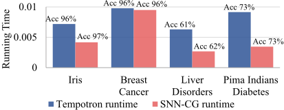
Effectiveness of joint learning. In SNN-CG, network connections and link weights are jointly learned in the iterative training scheme. To verify the benefit of joint learning, we compare SNN-CG with single Tempotron and STDPbased learning methods. The results are shown in Table. 3. Overall, the SNN-CG method outperforms both of Tempotron and STDP algorithms. Compared with the STDP method, the SNN-CG model achieves significantly better performances with 7%-18% improvement in accuracies. Compared with the classical Tempotron, our method obtains slightly better accuracies with much lower computational costs. As shown in Fig. 4, the SNN-CG method outperforms the classical Tempotron with better accuracies and lower computational costs. Since the SNN-CG reduces the number of connections in the network, the feedforward computation becomes more efficient.
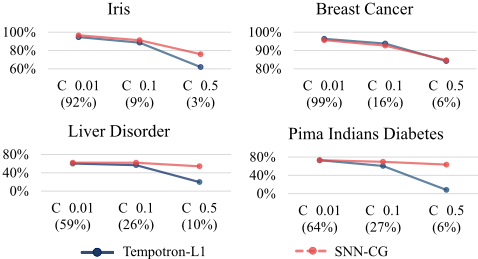
Effectiveness of connection learning. To demonstrate the strength of STDP-based connection learning, we compare SNN-CG with Tempotron using L1 norm regularization, denoted as Tempotron-L1. With the L1-regularization, the weights are more prone to zeros. As illustrated in Fig. 3, compared with the Tempotron-L1 method, the SNN-CG obtains better performance. We further compare the SNN-CG and Tempotron-L1 with different sparsity. As shown in Fig. 5, compared with Tempotron-L1, the SNN-CG method achieves better performance, especially in the high connection sparsity.
Comparison with existing methods. To evaluate the capability of SNN-CG, we compare our method with SVM, SpikeProp [Bohte et al., 2002], and ASA [Xie et al., 2017]. As illustrated in Table. 3, for the Iris dataset, we achieves 97% which is higher than SpikeProp (96%) and ASA (95%), and slightly lower than SVM (99%). For the Liver Disorder and the Pima Indians Diabetes datasets, SNN-CG achieves higher accuracies of 65% and 74%. For the Breast Cancer dataset, both SNN-CG and SpikeProp obtain the highest accuracy of 97%, while those of the SVM and ASA are 96% and 95%.
4 Conclusions
This paper proposed a spiking neural network with connection gates (SNN-CG) to jointly learn the connections and the link weights in SNN. The connection structures were optimized by the STDP rule with timing information, and the link weights were optimized by a supervised algorithm. Our method was evaluated on four benchmark datasets. The SNNCG method outperformed other supervised learning rules in SNN, and the SVM classifier. Experimental results demonstrated that, the joint learning of the connections and link weights improved the strength of SNN models with higher performance and lower computational costs.
Acknowledgments
This work was partly supported by the grants from National Natural Science Foundation of China (No. 61673340), National Key Research and Development Program of China (2017YFB1002503), and Zhejiang Provincial Natural Science Foundation of China (LZ17F030001, LR15F020001).
@inproceedings{ijcai2018p221,
  title     = {Jointly Learning Network Connections and Link Weights in Spiking Neural Networks},
  author    = {Qi, Yu and Shen, Jiangrong and Wang, Yueming and Tang, Huajin and Yu, Hang and Wu, Zhaohui and Pan, Gang},
  booktitle = {Proceedings of the Twenty-Seventh International Joint Conference on
               Artificial Intelligence, {IJCAI-18}},
  publisher = {International Joint Conferences on Artificial Intelligence Organization},
  editor    = {Jérôme Lang},
  pages     = {1597--1603},
  year      = {2018},
  month     = {7},
  note      = {Main track},
  doi       = {10.24963/ijcai.2018/221},
  url       = {https://doi.org/10.24963/ijcai.2018/221},
}
TY - CPAPER TI - Jointly Learning Network Connections and Link Weights in Spiking Neural Networks AU - Qi, Yu AU - Shen, Jiangrong AU - Wang, Yueming AU - Tang, Huajin AU - Yu, Hang AU - Wu, Zhaohui AU - Pan, Gang T2 - Proceedings of the Twenty-Seventh International Joint Conference on Artificial Intelligence, IJCAI-18 PB - International Joint Conferences on Artificial Intelligence Organization PY - 2018 SP - 1597 EP - 1603 DO - 10.24963/ijcai.2018/221 UR - https://doi.org/10.24963/ijcai.2018/221 ER -Copied
Machine-readable versions of this paper, for tools and AI agents:





