
Matrix Factorization with Scale-Invariant Parameters
Proceedings of the Twenty-Fourth International Joint Conference on Artificial Intelligence. Special Track on Machine Learning. Pages 4017-4023.
Abstract
Tuning hyper-parameters for large-scale matrix factorization (MF) is very time consuming and sometimes unacceptable. Intuitively, we want to tune hyper-parameters on small sub-matrix sample and then exploit them into the original large-scale matrix. However, most of existing MF methods are scale-variant, which means the optimal hyper-parameters usually change with the different scale of matrices. To this end, in this paper we propose a scale-invariant parametric MF method, where a set of scale-invariant parameters is defined for model complexity regularization. Therefore, the proposed method can free us from tuning hyper-parameters on large-scale matrix, and achieve a good performance in a more efficient way. Extensive experiments on real-world dataset clearly validate both the effectiveness and efficiency of our method.
- [Bach et al., 2008] Francis Bach, Julien Mairal, and Jean Ponce. Convex sparse matrix factorizations. arXiv preprint arXiv:0812.1869, 2008.
- [Blei et al., 2010] David M Blei, Perry R Cook, and Matthew Hoffman. Bayesian nonparametric matrix factorization for recorded music. In ICML '10, pages 439-446, 2010.
- [Bouchard et al., 2013] Guillaume Bouchard, Dawei Yin, and Shengbo Guo. Convex collective matrix factorization. In AISTATS '13, pages 144-152, 2013.
- [Boyd and Vandenberghe, 2009] Stephen Boyd and Lieven Vandenberghe. Convex optimization. Cambridge univer- sity press, 2009.
- [Candes and Plan, 2010] Emmanuel J Candes and Yaniv Plan. Matrix completion with noise. Proceedings of the IEEE, 98(6):925-936, 2010.
- [Candès and Recht, 2009] Emmanuel J Candès and Ben- jamin Recht. Exact matrix completion via convex op- timization. Foundations of Computational mathematics, 9(6):717-772, 2009.
- [Chan et al., 2013] Simon Chan, Philip Treleaven, and Licia Capra. Continuous hyperparameter optimization for large- scale recommender systems. In BigData '13, pages 350- 358, 2013.
- [Ding et al., 2010] Nan Ding, Rongjing Xiang, Ian Molloy, Ninghui Li, et al. Nonparametric bayesian matrix fac- torization by power-ep. In AISTATS '10, pages 169-176, 2010.
- [Freudenthaler et al., 2011] Christoph Freudenthaler, Lars Schmidt-Thieme, and Steffen Rendle. Bayesian factoriza- tion machines. 2011.
- [Ge et al., 2011] Yong Ge, Qi Liu, Hui Xiong, Alexander Tuzhilin, and Jian Chen. Cost-aware travel tour recom- mendation. In KDD '11, pages 983-991, 2011.
- [Hazan, 2008] Elad Hazan. Sparse approximate solutions to semidefinite programs. In LATIN 2008: Theoretical Infor- matics, pages 306-316. Springer, 2008.
- [Jaggi et al., 2010] Martin Jaggi, Marek Sulovsk, et al. A simple algorithm for nuclear norm regularized problems. In ICML '10, pages 471-478, 2010.
- [Journée et al., 2010] Michel Journée, Francis Bach, P-A Absil, and Rodolphe Sepulchre. Low-rank optimization on the cone of positive semidefinite matrices. SIAM Jour- nal on Optimization, 20(5):2327-2351, 2010.
- [Koren et al., 2009] Yehuda Koren, Robert Bell, and Chris Volinsky. Matrix factorization techniques for recom- mender systems. Computer, 42(8):30-37, 2009.
- [Koren, 2008] Yehuda Koren. Factorization meets the neigh- borhood: a multifaceted collaborative filtering model. In KDD '08, pages 426-434, 2008.
- [Lim and Teh, 2007] Yew Jin Lim and Yee Whye Teh. Vari- ational bayesian approach to movie rating prediction. In Proceedings of KDD Cup and Workshop, volume 7, pages 15-21, 2007.
- [Miller et al., 2003] Bradley N Miller, Istvan Albert, Shy- ong K Lam, Joseph A Konstan, and John Riedl. Movielens unplugged: experiences with an occasionally connected recommender system. In IUI '03, pages 263-266, 2003.
- [Mnih and Salakhutdinov, 2007] Andriy Mnih and Ruslan Salakhutdinov. Probabilistic matrix factorization. In NIPS '07, pages 1257-1264, 2007.
- [Pilászy et al., 2010] István Pilászy, Dávid Zibriczky, and Domonkos Tikk. Fast als-based matrix factorization for explicit and implicit feedback datasets. In RecSys '10, pages 71-78, 2010.
- [Rendle, 2010] Steffen Rendle. Factorization machines. In ICDM '10, pages 995-1000. IEEE, 2010.
- [Rendle, 2013] Steffen Rendle. Scaling factorization ma- chines to relational data. In VLDB '13, pages 337-348, 2013.
- [Rennie and Srebro, 2005] Jasson DM Rennie and Nathan Srebro. Fast maximum margin matrix factorization for col- laborative prediction. In ICML '05, pages 713-719, 2005.
- [Salakhutdinov and Mnih, 2008] Ruslan Salakhutdinov and Andriy Mnih. Bayesian probabilistic matrix factorization using Markov chain Monte Carlo. In ICML '08, vol- ume 25, 2008.
- [Srebro et al., 2003] Nathan Srebro, Tommi Jaakkola, et al. Weighted low-rank approximations. In ICML '03, vol- ume 3, pages 720-727, 2003.
- [Wu et al., 2012] Le Wu, Enhong Chen, Qi Liu, Linli Xu, Tengfei Bao, and Lei Zhang. Leveraging tagging for neighborhood-aware probabilistic matrix factorization. In CIKM '11, pages 1854-1858, 2012.
- [Xu et al., 2012] Minjie Xu, Jun Zhu, and Bo Zhang. Non- parametric max-margin matrix factorization for collabora- tive prediction. In NIPS '12, pages 64-72, 2012.
- [Yuan and Zhang, 2013] Xiao-Tong Yuan and Tong Zhang. Truncated power method for sparse eigenvalue problems. The Journal of Machine Learning Research, 14(1):899- 925, 2013.
- [Zhu et al., 2014] Hengshu Zhu, Enhong Chen, Hui Xiong, Kuifei Yu, Huanhuan Cao, and Jilei Tian. Mining mobile user preferences for personalized context-aware recom- mendation. ACM Trans. Intell. Syst. Technol., 5(4):58:1- 58:27, December 2014.
References were extracted automatically from the PDF and may contain errors.
Full text extracted automatically from the PDF; figures, tables and equations may differ. The PDF is the version of record.
1 Introduction
Matrix Factorization (MF) is among the most important machine learning techniques for real-world Collaborative Filtering (CF) applications, which attracts more and more attention in recent years [Koren et al., 2009; Ge et al., 2011; Wu et al., 2012; Zhu et al., 2014]. The main idea behind MF is that an m × n user-item rating matrix, where n items is assigned to m users, is modeled by the product of an m×K user factor matrix and the transpose of an n ×K item factor matrix [Srebro et al., 2003; Rennie and Srebro, 2005].
A variety of effective MF methods have been proposed, which can be mainly grouped into non-convex methods [Mnih and Salakhutdinov, 2007; Pil´aszy et al., 2010; 2010] and convex methods [Bach et al., 2008; Journ´ee et al., 2010; Bouchard et al., 2013]. The main difference between these two types of methods is that the number of factors can be self-determined in convex methods while it has to be set manually in non-convex methods. Indeed, both previous convex and non-convex methods can achieve good performance through carefully tuning their hyper-parameters. However, the cost of tuning hyper-parameters is often ignored. In fact, tuning hyper-parameters for large-scale MF problems is very time consuming and sometimes unacceptable [Chan et al., 2013]. Intuitively, a straightforward solution to this problem is to tune the hyper-parameters on small sub-matrix and then directly exploit them into the original large matrix. However, most of existing MF methods cannot work well for this idea due to the fact that their hyper-parameters are sensitive to the scale of matrix. In other words, the optimal hyper-parameters usually change with the different scale of matrices. We will both theoretically and experimentally analyze this issue in Section 5 and Section 6, respectively.
∗Corresponding author.
To address the above challenge, in this paper we propose a scale-invariant parametric MF method for facilitating model selection. Specifically, we assume that: the k-th latent factor values of any rating matrix and its sub-matrices follow the same normal distribution N(0, σ2 k ). With this assumption, we can first estimate a set of suitable {σ2 k }Kk=1 , namely Factorization Variances, by a randomly drawn sub-matrix. Then we use them as constraint parameters to formulate a new MF problem such that the variance of the k-th dimension latent factor values is not bigger than σ2 k , which can be used to conduct MF for the original large-scale matrix and any of its submatrices. Since the latent factor values of the sub-matrix and the original matrix are generated from the same distributions, we may still get a good performance on the original large matrix. In this process, factorization variances can introduce the similar effect of model complexity regularization, which is irrelevant to the scale of training matrices. In this sense, the proposed method is Scale-Invariant, which can free us from tuning hyper-parameters on large-scale matrix and achieve a good performance in a more efficient way. Specifically, our contributions can be summarized as follows.
First, to the best of our knowledge, we are the first to formulate the problem of MF with scale-invariant parameters. The unique perspective to this problem is to use the variance of the latent factor values from each dimension to control model complexity. All these parameters can be estimated on the resultant latent matrix output from any previous MF method on a random-sampled sub-matrix.
Second, we find that the formulated problem can be transformed into an equivalent problem, where the feasible set for each factor dimension is within a sphere. To solve this problem, we first initialize each dimension with the steepest decent eigenvector of the gradient matrix of the objective function. Then, we optimize the factors by the gradient decent method with projection to the feasible set.
Third, we both theoretically and experimentally prove that previous MF methods (i.e., in the form of both trace trade-off and trace bounding) are scale-variant. Moreover, extensive experiments on a real-world data set also empirically prove the effectiveness of our method, i.e., the hyper-parameters tuned by small sub-matrix can still achieve good performance on the original large-scale matrix.
2 Preliminaries &Assumption
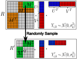
In this paper, we follow the Positive Semi-Definite (PSD) style MF model [Bach et al., 2008; Cand`es and Recht, 2009], which is shown in the top of Figure 1. Indeed, it is also equivalent to those SVD style formulations for MF [Mnih and Salakhutdinov, 2007; Koren, 2008]. Specifically, with PSD formulation the input matrix M = UV T ∈ Rm×n is put at the top-right corner of the PSD matrix R, and M T is put at the bottom-left corner of R. Here, we aim to solve the factorization problem R = Y Y T , where the top part of Y equals to U, and the bottom part of Y equals to V .
Different with previous studies, in this paper we consider the shared property among the column values of Y , and characterize the values in Y in a more sophisticated way. Specifically, we assume the values of the k-th column of Y satisfy the following distribution:
As we can see, values lie in the same column (e.g., the kth column) share a same variance σ2 k , and the {σ2 k }Kk=1 are named Factorization Variances. In particular, we assume:
Assumption 2.1. The factorization variances {σ2 k }Kk=1 are scale-invariant for MFs on different sized sub-matrices which are randomly drawn from the same matrix.
In other words, in our approach, the sampled sub-matrices share the same factorization variances with the original large matrix (i.e., as shown in Figure 1). With the above assumption, we can estimate a set of optimal parameters {σ2 k }Kk=1 on the sampled small sub-matrix M ′ , which is relatively efficient. Since the latent matrix Y and Y ′ are generated from the same distributions, we can exploit the estimated {σ2 k }Kk=1 into the original large matrix M and hopefully obtain comparable performance. Along this line, there are two major challenges:
- How to utilize the scale-invariant parameters, i.e, factorization variances, for large-scale MF?
- How to estimate the factorization variances (including the number of factors, namely K)?
None of the two challenges is trivial task. For the first one, we will propose a new problem, matrix FActorization with factorization VAriances (FAVA for short), with the factorization variances as the constraints, and solve it in Section 3. Furthermore, the second one will be discussed in Section 4.
3 MF with Factorization Variances
In this section, we assume the factorization variances {σ2 k }Kk=1 are known in advance. The estimation method for them will be detailed in Section 4.
3.1 The Formulation of FAVA
Here, we introduce how to adapt the factorization variances as the constraints for MF process. Specifically, in order to utilize the Assumption 2.1, we impose the following constraints:
The intuition behind these constraints is that we let the variance of the k-th column elements no larger than the known factorization variance. In these constraints, {σ2 k }Kk=1 serve as the model complexity controllers. The bigger the value of {σ2 k }Kk=1 is, the more freedom the values of the corresponding column have. Thus, it actually defines the feasible set for searching solution and guarantees the generalization ability of the model. With these constraints, we formulate the FAVA problem as follows:
where Yi,: means the i-th row of matrix Y . In order to turn the contraints into a consistent form, we let:
and then we can rewrite the variable Y as follows:
where P ∈ RN×K . Then, it is obvious that the constraints in Equation (2) are equivalent to ||P:,k||2 ≤ N, where P:,k means the k-th column of P, k = 1, ...,K. Then, we get the following equivalent form of FAVA:
If the above problem is solved, we can get Y = PΣK immediately. However, there are still some challenges:
- Firstly, simple gradient based method could not guarantee the searched solutions always meet the constraints of in Equation (6).
- Secondly, how to initialize the values of P? Randomly initialization can be a solution, but far from the best.
Next we will first show how we search solution for problem in Equation (6) in Section 3.2, then we give an effective initialization method for P in Section 3.3.
3.2 Sphere Projection for FAVA
As we can see in the constrains of problem in Equation (6), the P:,k is within a ball with radius √N and its sphere, we optimize the latent factors by gradient decent method with projection to the feasible set of FAVA. Firstly, the gradient of objective function in Equation (6) is:
from above we also know that:
Assume αt is the t-th iteration decent step size, then we update each column P:,k by the following rule:
where
As the projection only happens when tr(P ′ :,k P ′ :,k T ) > N, and the projection makes P ′ :,k project onto the sphere of ball with radius √N in RN . Thus, we call this method Sphere Projection. In addition, the step size αt can be searched by the binary search method BiSearch(P (t) , △P (t) ) as follows:
- Set αt = 1.0;
- Update each column of P (t) by Equation (9) and the result is denoted as P (t+1) ;
Finally, we stop the optimization iteration when αt < ε, where ε is a given accuracy level.
3.3 Steepest Initialization for FAVA
In this subsection, we will show the process that initializes columns of P with eigendecomposition of gradient matrix ∇XG(X). The intuition behind this process is that we initialize the columns of P with the first K steepest decent direction of G(X) at X = 0.
Firstly, by the definition in Equation (6), we know that ∇XG(X) is always a symmetric matrix of the block form
in [Jaggi et al., 2010], we have the following proposition:
Proposition 3.1. The spectrum of ∇XG(X) is always symmetric: whenever [ uv ] is an eigenvector for some eigenvalue
is an eigenvector for -ρ.
So we know that the smallest eigenvalue of ∇XG(X) is always ρmin ≤ 0. Then we have the following theorem.
Theorem 3.2. Given Yk ∈ RN×k , let Yk+1 = [Yk|√β · ⃗y] ∈ RN×(k+1) , where β ∈ R+, ⃗y ∈ RN and ||⃗y|| = 1, ⃗y is called attached vector for Yk. Then, the unit eigenvector ⃗ymin for the smallest eigenvalue ρmin of ∇XG(YkY T k ) is the steepest decent attached vector of Yk, which means that f(β, ⃗y) = G(Yk+1Y T k+1 ) decent the fastest when ⃗y = ⃗ymin at β = 0.
Proof. Firstly, let Xk = YkY T k and △X = ⃗y⃗yT . By definition we have:
Then we have:
where A ◦ B = tr(AB). Finally we have:
And we also know that:
which means f(β, ⃗y) is decent at β = 0 when ⃗y = ⃗ymin, and for any ⃗y ̸= 0 and ||⃗y|| = 1 we have:
⃗ymin is the steepest decent attached vector of Yk is proved.
After we getting the steepest decent attached vector, now we focus on how to get the steepest step size β. Actually, that is quite straight forward, let Xk = YkY T k and△Xmin = ⃗ymin⃗yTmin . By Equation (12), let f ′β (β, ⃗ymin) = 0, then:
where IΩ is a matrix that when (i, j) ∈ Ω, IΩ(i, j) = 1, else IΩ(i, j) = 0, and A ⊙ B = C means Ci,j = Ai,j × Bi,j. Then we immediately have:
Now, we can summarize the eigenvector initialization method EigenInitial(R, {σk}Kk=1 ) for P as follows:
- Find {ρmin, ⃗ymin} of matrix ∇XG(Xk);
- Compute β by Equation (17), let k = k + 1;
- Let β′ = √β σk when √β σk ≤ √N, else β′ = √N;
- Let Pk = [Pk-1|β′ · ⃗ymin];
- Let Σk = diag{σ1, ..., σk}, Yk = PkΣk, Xk = YkY T k ;
- Repeat 2 to 7 until k = K;
- Return P = PK.
In addition, line 4 is to ensure the initial values of P meet the constraints of problem in Equation (6). Line 2 is to find {ρmin, ⃗ymin} of matrix ∇XG(Xk), we do not need to conduct full eigendecomposition to the matrix ∇XG(Xk) as it is very time consuming which does not fit for sparse large scale matrix, we can use the sparse power method [Yuan and Zhang, 2013] with a shift to the original matrix ∇XG(Xk). Let c be a constant large enough, we construct a shifted matrix D = c · I -∇XG(Xk), then we can easily get the dominant eigen value-vector pair {ρd, ⃗yd} of matrix D through a few power iterations (less than 20 with accuracy level 10-5 in most circumstances), then we get {ρmin = c - ρd, ⃗y = ⃗yd}. Finally, we summarize the FAVA method in Algorithm 1.
Algorithm 1 Scale-Invariant Matrix Factorization (FAVA).
Input:
Accuracy level ε, Incomplete matrix R;
Factorization Variances {σ2 1 , σ2 2 , ..., σ2K };
Output: Y ;
- 1: Let P = EigenInitial(R, {σk});
- 2: Let t = 0, αt = 10 × ε and P (t) = P ;
- 3: while αt ≥ ε do
- 4: Compute △P (t) by Equation (7);
- 5: Let αt+1 = BiSearch(P (t) ,△P (t) );
- 6: Update each column of P (t) by Equation (9), and the result is denoted as P (t+1) ;
- 7: t = t + 1;
- 8: end while
- 9: return Y = P (t)ΣK.
4 Estimating Factorization Variances
In this section, we discuss about how to estimate the Factorization Variances and also the number of them, i.e.,K. Before getting into the detail, it is worth mentioning that the algorithms introduced in this section are only applied to small sampled sub-matrices for estimating suitable factorization variances through hyper-parameter tuning.
As the number of factors of non-convex methods must be set manually, we focus our discussion on using convex methods for estimating factorization variances. The most widely used two forms of convex formulation are the trace trade-off form [Bach et al., 2008; Candes and Plan, 2010]:
and the trace bounding form [Hazan, 2008; Jaggi et al., 2010]:
Actually, as mentioned in [Jaggi et al., 2010], the above two formulations are equivalent in the following sense.
Theorem 4.1. If X is an optimal solution to Problem in Equation (18), let γ = tr(X), then X is also an optimal solution to Problem in Equation (19). On the other hand, if X is an optimal solution to Problem in Equation (19), let λ = - ∇XG(X)◦X tr(X) , then X is also an optimal solution to Problem in Equation (18).
Next, we choose the formulation form of trace trade-off in Equation (18) as an example to discuss its solution. Firstly, let X = Y Y T , then the constraint in Equation (18) is canceled and the problem can be rewritten into a non-convex form [Mnih and Salakhutdinov, 2007] (with λ = λu = λv):
Then, we use the method proposed in [Journ´ee et al., 2010] to solve this problem in Equation (18) through finding the local optimum of the problem in Equation (20), and increasing the number of Y 's columns one by one until the condition of the following Theorem 4.2 is met to achieve its global optimum.
Theorem 4.2. A local minimizer Y of the non-convex problem in Equation (20) provides a global minimum point X = Y Y T of the convex problem in Equation (18) if and only if SY = ∇XF (Y Y T ) ⪰ 0.
After we get Y , X = Y Y T is the global optimum for Problem in Equation (18). Then, by the assumption in Equation (1), we can approximate the factorization variances {σ2 k }Kk=1 as follows:
On the small sampled sub-matrix we can tune the best parameter λ∗ for Problem in Equation (18) by cross-validation. Then, with the latent factors resulted from λ∗ we can estimate the corresponding factorization variances. Hopefully, these factorization variances work well on the original large matrix. The experiments will empirically validate this.
5 Theoretical Analysis on Scale-Variant and Scale-Invariant Methods
Now, we give the theoretical analysis on the relationship between the scale-invariant formulation FAVA (proposed in this paper) and the scale-variant ones (in the form of both trace trade-off and trace bounding).
Firstly, let's take a look at the relationship between FAVA and the trace trade-off formulation. Before detailing this relationship, we need to first present the following two lemmas.
Lemma 5.1. X is an optimal solution of problem in Equation (18) if and only if the following conditions hold:
where S = ∇XF (X).
Lemma 5.2. If P is a local minimum solution of problem in Equation (6), then the following conditions hold:
where △P is the gradient of objective function in Equation (6), and △P:,k means the k-th column of △P .
The conditions in Lemma 5.1 are the KKT conditions of the problem in Equation (18) and similarly the conditions in Lemma 5.2 are the KKT conditions of the problem in Equation (6) (see [Boyd and Vandenberghe, 2009]).
Theorem 5.3. Let Y = PΣK, where P is a local minimum solution of FAVA in Equation (6), and X = Y Y T . If X is an optimal solution to problem in Equation (18) for some λ, then we have:
Proof. Firstly, we know that F(X) = G(X)+λtr(X), then by 3# of Lemma 5.1 we know that:
Both sides of the above equation get trace, then we have:
And by constraints in Equation (2) we also know that:
Next, we prove ∇XG(X) ◦ X ≤ 0. As X = Y Y T and Y = PΣK, then we have:
By Equation (7) we have:
By conditions in Lemma 5.2 we have:
Now we have already proved:
Theorem 5.3 clarifies the correlation between FAVA and the trace trade-off form for MF. It actually provides a lower bound for the parameter λ by considering the equivalence of the two problems. We can clearly see that this lower bound on λ is not only dependant on the scale of the matrix N, but also the sparsity of the incomplete matrix R (the number of non-zero terms in ∇XG(X) ◦ X is |Ω|). That is the reason why the best working λ∗ on a sub-matrix may not perform well on large scale matrices. Similarly, we show the correlation between FAVA and bounding trace formulation with the following theorem.
Theorem 5.4. Let Y = PΣK, where P is a local minimum solution of FAVA in Equation (6), and X = Y Y T . If X is an optimal solution for problem in Equation (19) for some γ, then we have:
The above theorem can be got immediately by the bounding trace constraint in Equation (19), as N ∑Kk=1 σ2 k is the upper bound of tr(X) by the constraints in Equation (6). It states that the parameter γ is also dependant on the scale of the matrix N. This is the reason why the best working γ ∗ on a sub-matrix may not perform well on large matrices.
6 Experiment
In this section, we validate the effectiveness and efficiency of our approach FAVA based on a real-world dataset.
Baselines. We choose two widely used convex MF methods for comparison, namely
TTF: Trace Trade-off Form [Bach et al., 2008; Bouchard et al., 2013], which is formulated in Equation (18).
TBF: Trace Bounding Form [Hazan, 2008; Jaggi et al., 2010], which is formulated in Equation (19).
In the experiments, FAVA uses TTF to estimate the {σ2 k }Kk=1 by randomly drawn sub-matrix and operates on the target matrix. The convergence level of all methods is set to 10-5 .
| Dataset | m | n | #rating | Dataset | m | n | #rating |
|---|---|---|---|---|---|---|---|
| M0.04,1 | 179 | 124 | 4,126 | M0.08,1 | 899 | 319 | 27,858 |
| M0.04,2 | 182 | 126 | 4,091 | M0.08,2 | 1,092 | 356 | 35,547 |
| M0.04,3 | 197 | 123 | 4,475 | M0.08,3 | 902 | 363 | 28,769 |
| M0.04,4 | 184 | 143 | 4,521 | M0.08,4 | 922 | 326 | 28,852 |
| M0.04,5 | 126 | 105 | 2,584 | M0.08,5 | 899 | 337 | 27,246 |
| M0.16,1 | 3,930 | 928 | 176,117 | ||||
| M0.16,2 | 3,422 | 864 | 144,552 | Dataset | MovieLens10M | ||
| M0.16,3 | 3,297 | 841 | 136,066 | m | 69,878 | ||
| M0.16,4 | 3,929 | 875 | 166,827 | n | 10,677 | ||
| M0.16,5 | 3,538 | 914 | 149,484 | #rating | 10,000,054 | ||
Dataset. Here we use MovieLens10M [Miller et al., 2003] dataset for validation. Specifically, we randomly splited the large dataset into training set and test set (80% for training, 20% for test). All the sub-matrices was sampled from the training set. Let M ∈ Rm×n be the original large scale matrix, we sampled each sub-matrix dataset as follows: given a ratio r, we randomly sampled m×r rows and n×r columns from the M first; then we collected the elements that are both covered by the sampled rows and columns into a set Ω; finally, we removed rows and columns whose numbers of elements in Ω are less than 10, and the remaining rows and columns and their covering elements in Ω formed our resulting sub-matrix dataset. For each ratio r, we sampled 5 submatrices independently, and the id-th sample is denoted as Mr,id. The statistics of datasets are summarized in Table 1. Unless otherwise noted, all methods conducted 5-fold crossvalidation when they run on the sub-matrix datasets.
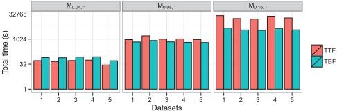
Overall comparison on sub-matrices. In this experiment, we tuned parameters for TTF and TBF on the sub-matrices first, let λ variate from 0.1 to 4.0 by step size 0.1, and γ ∈ {10, 20, 30, 40, 50, 60, 70, 80, 90, 100, 200, 300, 400, 500, 600, 700, 800, 900, 1000, 2000, 3000, 4000, 5000, 6000, 7000, 8000, 9000, 10000}. The left part of Table 2 shows the parameter tuning results. Then we used the best parameters estimated by M0.04,1 for all the methods, and let them run on all the sub-matrices, results are shown in the right part of Table 2. Figure 2 shows the total time of parameter tuning for both TTF and TBF methods.
As we can see from the right part of Table 2, for effectiveness comparison, FAVA performs the best across all sub-matrices. While for efficiency comparison, TTF method has superiority when the scale of sub-matrices is small (e.g., M0.04,∗ series sub-matrices). However, when the scale of sub-matrices become larger, the efficiency of TTF becomes worse rapidly under the parameter setting that are estimated by M0.04,1. In contrast, the efficiencies of TBF and FAVA are always comparable across all sub-matrices. It is worth to point out that although the results of FAVA are not as good as the best results of TTF and TBF on M0.08,∗ and M0.16,∗ series sub-matrices, together with Figure 2 we can see that the amount of running time of FAVA to achieve such results (i.e., TTF parameter tuning time on M0.04,1 + FAVA running time) is much less than the parameter tuning time of TTF and TBF on these sub-matrices. Also, from Figure 2 we can find the parameter tuning time grows enormously as the matrix scale increases, which indicates tuning parameter on largescale matrix is very time consuming.
Comparison on MovieLens10M. In this experiment, we used the best parameters estimated by M0.04,1 for all the methods, then let they run on the original large-scale MovieLens10M matrix (results are shown in Table 3). Then, we used the M0.04,1, M0.08,1 and M0.16,1 to estimate 3 different sets of {σ2 k }Kk=1 , and feed them into our FAVA method for MF on MovieLens10M dataset (results are shown in Table 4).
| TTFλ=1.0 | TBFγ=70.0 | FAVA | |||
|---|---|---|---|---|---|
| RMSE | Time | RMSE | Time | RMSE | Time |
| 0.92111 | 11516m5.600s | 1.0513 | 48m5.631s | 0.81530 | 95m21.948s |
From Table 3 we can see that, once again FAVA plays the best on effectiveness, i.e., its RMSE is much better than that of baselines. The efficiencies of TBF and FAVA are comparable, while that of TTF on MovieLens10M dataset is much worse than the other two methods. Moreover, from Table 4 we can see that the RMSE is almost unchange as the scale of sub-matrices changes, however, the running time of FAVA increases as the scale of sub-matrices becomes large. That is because when the scale of sub-matrices becomes larger and larger, the structure of matrix becomes more and more complex and the TTF method needs more latent factors to capture them, which leads to more computation cost for FAVA on the original MovieLens10M matrix.
| M0.04,1 | M0.08,1 | M0.16,1 | |||
|---|---|---|---|---|---|
| RMSE | Time | RMSE | Time | RMSE | Time |
| 0.81530 | 95m21.948s | 0.81513 | 180m26.588s | 0.81885 | 322m18.697s |
7 RelatedWork
We briefly review works about MF in terms of collaborative filtering here. Generally speaking, the MF methods can be divided into two categories, Bayesian (e.g., [Lim and Teh, 2007; Salakhutdinov and Mnih, 2008; Freudenthaler et al., 2011; Rendle, 2013] and non-Bayesian (e.g., [Mnih and Salakhutdinov, 2007; Pil´aszy et al., 2010; Rendle, 2010]) methods. The main difference between these two kinds of methods is that the Baysian methods introduce Baysian inference to the inferring of latent factors, while the non-Bayesian methods give MAP approximation to them. The method proposed in this paper belongs to the non-Bayesian method. All these methods can achieve good performance through carefully tuning their hyper-parameters. However, the cost of hyper-parameters tuning is ignored.
Although there are Baysian methods that claim they are non-parametric [Blei et al., 2010; Ding et al., 2010; Xu et al., 2012], they are only non-parametric on how to set the number of latent factors, they still have to tune hyper-parameters (e.g., regularization parameters, prior sampling distribution parameters) to a achieve good performance. Actually, the non-Baysian convex MF methods [Bach et al., 2008; Jaggi et al., 2010; Journ´ee et al., 2010; Bouchard et al., 2013] also can determine the number of latent factors automatically.
The proposed method is different from all these works. Firstly, to the best of our knowledge, we are the first to formulate a problem of MF with scale-invariant parameters. Secondly, we propose a new optimization problem called FAVA for scale-invariant parametric MF, and solve it both effectively and efficiently. Thirdly, we present the theoretical properties show that the previous MF methods (in the form of both trace trade-off and trace bounding) are scale-variant.
| Parameter Tuning | ||||
|---|---|---|---|---|
| Dataset | TTF | TBF | ||
| λbest | RMSE | γbest | RMSE | |
| M004,1 | 1.0 | 0.91507±0.02324 | 70.0 | 0.91689±0.02283 |
| M004,2 | 1.0 | 0.89232±0.02154 | 60.0 | 0.89327±0.02207 |
| M004,3 | 1.1 | 0.90167±0.02855 | 70.0 | 0.90265±0.02851 |
| M0.04,4 | 1 | 0.90275±0.01600 | 80.0 | 0.90511±0.01606 |
| M0.04,5 | 0.9 | 0.96147±0.03611 | 60.0 | 0.96256±0.03636 |
| M0.08,1 | 1.6 | 0.89540±0.00678 | 300.0 | 0.89663±0.00707 |
| M0.08,2 | 1.7 | 0.88941±0.00520 | 400.0 | 0.89083±0.00557 |
| M0.08,3 | 1.7 | 0.89779±0.00748 | 300.0 | 0.89910±0.00714 |
| M0.08,4 | 1.7 | 0.90125±0.00616 | 300.0 | 0.90278±0.00600 |
| M0.08,5 | 1.7 | 0.91429±0.00995 | 300.0 | 0.91552±0.00990 |
| M0.16,1 | 2.6 | 0.87246±0.00200 | 1000.0 | 0.87565±0.00200 |
| M0.16,2 | 2.4 | 0.86465±0.00283 | 1000.0 | 0.86686±0.00283 |
| M0.16,3 | 2.3 | 0.88353±0.00173 | 1000.0 | 0.88571±0.00200 |
| M0.16,4 | 2.5 | 0.87162±0.00346 | 1000.0 | 0.87421±0.00374 |
| M0.16,5 | 2.4 | 0.88460±0.00316 | 1000.0 | 0.88669±0.00332 |
| Parameters Estimated by M004,1 | |||||
|---|---|---|---|---|---|
| TTFλ=1.0 | TBFγ=70.0 | FAVA | |||
| RMSE | Time (s) | RMSE | Time (s) | RMSE | Time (s) |
| 0.91507±0.02324 | 1.656 | 0.91689±0.02283 | 4.276 | 0.90697±0.02317 | 2.466 |
| 0.89232±0.02154 | 1.538 | 0.89342±0.02182 | 4.204 | 0.88595±0.01709 | 2.382 |
| 0.90213±0.02877 | 1.679 | 0.90265±0.02851 | 4.685 | 0.89793±0.03421 | 2.590 |
| 0.90275±0.01600 | 1.818 | 0.90554±0.01568 | 4.78 | 0.89171±0.01470 | 2.531 |
| 0.96219±0.03662 | 0.830 | 0.96418±0.03567 | 2.767 | 0.95109±0.03162 | 1.294 |
| 0.91132±0.00640 | 37.66 | 0.93555±0.00872 | 30.816 | 0.90303±0.00387 | 25.438 |
| 0.89588±0.00548 | 71.006 | 0.93697±0.00424 | 36.022 | 0.88909±0.00387 | 35.524 |
| 0.91524±0.00700 | 40.108 | 0.93447±0.00831 | 33.47 | 0.90663±0.00000 | 26.953 |
| 0.91768±0.00520 | 40.927 | 0.94458±0.00700 | 28.437 | 0.90581±0.00424 | 25.942 |
| 0.92521±0.00975 | 36.897 | 0.94752±0.01082 | 27.05 | 0.92075±0.00906 | 24.901 |
| 0.91254±0.00200 | 948.059 | 0.99213±0.00245 | 174.225 | 0.88960±0.00245 | 233.074 |
| 0.90014±0.00283 | 613.385 | 0.97799±0.00424 | 140.29 | 0.88712±0.00141 | 174.156 |
| 0.91835±0.00245 | 597.935 | 0.99485±0.00245 | 129.596 | 0.90078±0.00447 | 180.950 |
| 0.90975±0.00346 | 854.419 | 0.99198±0.00424 | 163.595 | 0.89998±0.00316 | 256.393 |
| 0.92096±0.00316 | 687.802 | 0.99236±0.00245 | 144.217 | 0.90935±0.00500 | 222.723 |
8 Conclusion
In this paper, we proposed a scale-invariant parametric MF method for addressing the idea that tuning hyper-parameters on small sub-matrix and then use them on the original large scale matrix. Specifically, we can use any of the previous MF methods to estimate the best working factorization variances on small sampled sub-matrix, and then use them for the proposed method to conduct both effective and efficient MF on original large scale matrix. Extensive experiments also show that the proposed method can achieve good performance on the original large scale matrix with the estimated factorization variances on small sampled sub-matrix.
Acknowledgments
This research was partially supported by grants from the National Science Foundation for Distinguished Young Scholars of China (Grant No. 61325010), the National High Technology Research and Development Program of China (Grant No. 2014AA015203), the Fundamental Research Funds for the Central Universities of China (Grant No. WK2350000001) and the Natural Science Foundation of China (Grant No. 61403358). Ping Luo was supported by the National Natural Science Foundation of China (No. 61473274) and National 863 Program (No.2014AA015105).
@inproceedings{ijcai2015p564,
  title     = {Matrix Factorization with Scale-Invariant Parameters},
  author    = {Zeng, Guangxiang and Zhu, Hengshu and Liu, Qi and Luo, Ping and Chen, Enhong and Zhang, Tong},
  booktitle = {Proceedings of the Twenty-Fourth International Joint Conference on
               Artificial Intelligence, {IJCAI-15}},
  publisher = {International Joint Conferences on Artificial Intelligence},
  editor    = {Qiang Yang and Michael Wooldridge},
  pages     = {4017--4023},
  year      = {2015},
  month     = {7},
  note      = {Special Track on Machine Learning},
  url       = {https://ijcai.org/proceedings/2015/564},
}
TY - CPAPER TI - Matrix Factorization with Scale-Invariant Parameters AU - Zeng, Guangxiang AU - Zhu, Hengshu AU - Liu, Qi AU - Luo, Ping AU - Chen, Enhong AU - Zhang, Tong T2 - Proceedings of the Twenty-Fourth International Joint Conference on Artificial Intelligence, IJCAI-15 PB - International Joint Conferences on Artificial Intelligence PY - 2015 SP - 4017 EP - 4023 UR - https://ijcai.org/proceedings/2015/564 ER -Copied
Machine-readable versions of this paper, for tools and AI agents:





