
Scalable Maximum Margin Matrix Factorization by Active Riemannian Subspace Search
Proceedings of the Twenty-Fourth International Joint Conference on Artificial Intelligence. Special Track on Machine Learning. Pages 3988-3993.
Abstract
The user ratings in recommendation systems are usually in the form of ordinal discrete values. To give more accurate prediction of such rating data, maximum margin matrix factorization (M3F) was proposed. Existing M3F algorithms, however, either have massive computational cost or require expensive model selection procedures to determine the number of latent factors (i.e. the rank of the matrix to be recovered), making them less practical for large scale data sets. To address these two challenges, in this paper, we formulate M3F with a known number of latent factors as the Riemannian optimization problem on a fixed-rank matrix manifold and present a block-wise nonlinear Riemannian conjugate gradient method to solve it efficiently. We then apply a simple and efficient active subspace search scheme to automatically detect the number of latent factors. Empirical studies on both synthetic data sets and large real-world data sets demonstrate the superior efficiency and effectiveness of the proposed method.
- [Absil et al., 2008] P.-A. Absil, R. Mahony, and R. Sepulchre. Op- timization Algorithms on Matrix Manifolds. Princeton University Press, Princeton, NJ, USA, 2008.
- [Balzano et al., 2010] L. Balzano, R. Nowak, and B. Recht. Online identification and tracking of subspaces from highly incomplete information. In Proceedings of Allerton, 2010.
- [Bennett and Lanning, 2007] J. Bennett and S. Lanning. The netflix prize. In Proceedings of the KDD Cup Workshop 2007. ACM, 2007.
- [Boumal and Absil, 2011] N. Boumal and P.-A. Absil. Rtrmc: A riemannian trust-region method for low-rank matrix completion. In NIPS, 2011.
- [Candés and Plan, 2010] E. J. Candés and Y. Plan. Matrix comple- tion with noise. Proceedings of the IEEE, 98(6):925-936, 2010.
- [Candés and Recht, 2009] E. J. Candés and B. Recht. Exact ma- trix completion via convex optimization. Found. Comput. Math., 9:717-772, 2009.
- [Chang et al., 2015] Xiaojun Chang, Feiping Nie, Zhigang Ma, Yi Yang, and Xiaofang Zhou. A convex formulation for spec- tral shrunk clustering. In AAAI, 2015.
- [DeCoste, 2006] Dennis DeCoste. Collaborative prediction using ensembles of maximum margin matrix factorizations. In ICML. ACM, 2006.
- [Dror et al., 2012] G. Dror, N. Koenigstein, Y. Koren, and M. Weimer. The Yahoo! Music Dataset and KDD-Cup'11. JMLR Workshop and Conference Proceedings, 18:3-18, 2012.
- [Fazel, 2002] M. Fazel. Matrix rank minimization with applica- tions. 2002. PhD thesis, Stanford University.
- [Han et al., 2013] Yahong Han, Zhongwen Xu, Zhigang Ma, and Zi Huang. Image classification with manifold learning for out- of-sample data. Signal Processing, 93(8):2169-2177, 2013.
- [Herlocker et al., 1999] Jonathan L. Herlocker, Joseph A. Konstan, Al Borchers, and John Riedl. An algorithmic framework for per- forming collaborative filtering. In SIGIR. ACM, 1999.
- [Hsieh and Olsen, 2014] Cho-Jui Hsieh and Peder Olsen. Nuclear norm minimization via active subspace selection. In ICML, 2014.
- [Huang et al., 2013] Jin Huang, Feiping Nie, and Heng Huang. Ro- bust discrete matrix completion. In AAAI, 2013.
- [Karatzoglou et al., 2010] Alexandros Karatzoglou, Markus Weimer, and Alex J Smola. Collaborative filtering on a budget. In AISTATS, 2010.
- [Lin et al., 2010] Z. Lin, M. Chen, and Y. Ma. The augmented la- grange multiplier method for exact recovery of corrupted low- rank matrices. Technical report, UIUC, 2010.
- [Lu et al., 2013] Xinyan Lu, Fei Wu, Siliang Tang, Zhongfei Zhang, Xiaofei He, and Yueting Zhuang. A low rank structural large margin method for cross-modal ranking. In SIGIR, 2013.
- [Meyer et al., 2011] G. Meyer, S. Bonnabel, and R. Sepulchre. Lin- ear regression under fixed-rank constraints: A riemannian ap- proach. In ICML, 2011.
- [Mishra et al., 2012] B. Mishra, K. A. Apuroop, and R. Sepulchre. A riemannian geometry for low-rank matrix completion. Techni- cal report, 2012.
- [Mnih and Salakhutdinov, 2007] Andriy Mnih and Ruslan Salakhutdinov. Probabilistic matrix factorization. In NIPS, 2007.
- [Ngo and Saad, 2012] T. T. Ngo and Y. Saad. Scaled gradients on grassmann manifolds for matrix completion. In NIPS, 2012.
- [Nie et al., 2012] Feiping Nie, Heng Huang, and Chris Ding. Low- rank matrix recovery via efficient schatten p-norm minimization. In AAAI, 2012.
- [Recht et al., 2010] B. Recht, M. Fazel, and P. A. Parrilo. Guaran- teed minimum rank solutions to linear matrix equations via nu- clear norm minimization. SIAM Rev., 52(3), 2010.
- [Recht et al., 2011] Benjamin Recht, Christopher Re, Stephen Wright, and Feng Niu. Hogwild: A lock-free approach to par- allelizing stochastic gradient descent. In NIPS, 2011.
- [Rennie and Srebro, 2005] Jasson D. M. Rennie and Nathan Sre- bro. Fast maximum margin matrix factorization for collaborative prediction. In ICML, 2005.
- [Srebro et al., 2005] Nathan Srebro, Jason D. M. Rennie, and Tommi S. Jaakola. Maximum-margin matrix factorization. In NIPS. MIT Press, 2005.
- [Su and Khoshgoftaar, 2009] Xiaoyuan Su and Taghi M. Khosh- goftaar. A survey of collaborative filtering techniques. Adv. in Artif. Intell., 2009:4, 2009.
- [Tan et al., 2014] Mingkui Tan, Ivor W. Tsang, Li Wang, Bart Van- dereycken, and Sinno Jialin Pan. Riemannian pursuit for big ma- trix recovery. ICML, 2014.
- [Toh and Yun, 2010] Kim-Chuan Toh and Sangwoon Yun. An ac- celerated proximal gradient algorithm for nuclear norm regular- ized linear least squares problems. Pacific Journal of Optimiza- tion, 6:615-640, 2010.
- [Vandereycken, 2013] Bart Vandereycken. Low-rank matrix com- pletion by riemannian optimization. SIAM J. Optim., 23(2):1214- 1236, 2013.
- [Weimer et al., 2007] Markus Weimer, Alexandros Karatzoglou, Quoc Viet Le, and Alex Smola. Maximum margin matrix fac- torization for collaborative ranking. NIPS, 2007.
- [Weimer et al., 2008] Markus Weimer, Alexandros Karatzoglou, and Alex Smola. Improving maximum margin matrix factoriza- tion. Machine Learning, 72(3):263-276, 2008.
- [Wen et al., 2012] Z. Wen, W. Yin, and Y. Zhang. Solving a low- rank factorization model for matrix completion by a non-linear successive over-relaxation algorithm. Math. Program. Comput., 4(4):333-361, 2012.
- [Wu, 2007] Mingrui Wu. Collaborative filtering via ensembles of matrix factorizations. In Proceedings of KDD Cup and Work- shop, 2007.
- [Xiao et al., 2014] Shijie Xiao, Mingkui Tan, and Dong Xu. Weighted block-sparse low rank representation for face cluster- ing in videos. In ECCV, 2014.
- [Xiao et al., 2015] Shijie Xiao, Wen Li, Dong Xu, and Dacheng Tao. FaLRR: A Fast Low Rank Representation Solver. In CVPR, 2015.
- [Xu et al., 2012] Minjie Xu, Jun Zhu, and Bo Zhang. Nonparamet- ric max-margin matrix factorization for collaborative prediction. In NIPS, 2012.
- [Xu et al., 2013] Minjie Xu, Jun Zhu, and Bo Zhang. Fast max- margin matrix factorization with data augmentation. In ICML, 2013.
- [Yang et al., 2013] Yi Yang, Zhigang Ma, A.G. Hauptmann, and N. Sebe. Feature selection for multimedia analysis by sharing information among multiple tasks. Multimedia, IEEE Transac- tions on, 15(3):661-669, April 2013.
References were extracted automatically from the PDF and may contain errors.
Full text extracted automatically from the PDF; figures, tables and equations may differ. The PDF is the version of record.
1 Introduction
The rapid increase of Web services has witnessed an increasing demand for predicting the preferences of users on products of interest, such as movies and music tracks [Su and Khoshgoftaar, 2009]. This task, also known as the collaborative filtering (CF), is a principal task in recommender systems [Weimer et al., 2008; Huang et al., 2013]. In general, the user ratings are given in discrete values, including binary ratings and ordinal ratings [Srebro et al., 2005]. The binary ratings can be either "+1" (like) or "-1" (dislike); while the ordinal ratings are in discrete values such as 1-5 "stars", which are more popular in applications.
Given a small number of user ratings Y ∈ Rm×n (from m users on n items), the aim of CF is to reconstruct the unobserved ratings. Let Ω be a subset containing the indices of the observed entries. To perform the reconstruction, a common approach is to learn a low-rank matrix X to fit Y by solving the following optimization problem:
∗The corresponding author.
where k denotes the number of latent factors (i.e. the rank of X) and f(X) denotes some loss functions. The low-rank property has been studied in a variety of applications [Xiao et al., 2014; 2015; Yang et al., 2013]. In many studies, such as matrix completion, the least-square loss function f(X) = ∑ij∈Ω(Xij - Yij)2 is used [Cand´es and Recht, 2009; Cand´es and Plan, 2010; Vandereycken, 2013]. Despite of its popularity, the least-square loss may not perform well when the ratings are discrete values [Srebro et al., 2005].
To deal with rating data, the maximum margin matrix factorization (M3F) is proposed using the hinge loss [Srebro et al., 2005; Rennie and Srebro, 2005; Weimer et al., 2008]. For binary ratings, the objective function can be written as
where h(z) = max(0, 1 - z). The hinge loss h(z) for binary ratings can be easily extended to general ordinal ratings where Yij ∈ {1, 2, ...L} by applying L + 1 thresholds θ0 ≤ θ1 ≤ ... ≤ θL learned from data [Rennie and Srebro, 2005]. For the discrete valued rating data, hinge loss would achieve better performance compared to the least square loss.
Problem (1) is known to be NP-hard. Many researchers [Fazel, 2002; Recht et al., 2010] thus propose to solve its nuclear-norm convex relaxation minXλ||X||∗ + f(X), where ||X||∗ denotes the nuclear norm of X and λ is a regularization parameter. Many convex optimization methods, such as proximal gradient methods [Toh and Yun, 2010; Nie et al., 2012] can be adopted to solve this problem. However, these methods may scale poorly due to the requirement of singular value decompositions (SVDs) of large ranks.
To improve the scalability, some researchers assumes that the rank of X (i.e. k) is known, and X can be explicitly factorized as X = UV⊤, where U ∈ Rn×k and V ∈ Rm×k [Rennie and Srebro, 2005; Mnih and Salakhutdinov, 2007]. They then solve the following variational formulation instead:
where λ is a regularization parameter. Many methods, such as the stochastic gradient descent (SGD), can be used to solve this problem. However, in real applications, the prior knowledge about k is not likely accessible. Consequently, these algorithms may have to perform expensive model selections to determine k, which is unaffordable in computation [Xu et al., 2012; 2013]. Additionally, since problem (3) is non-convex w.r.t. U and V simultaneously, most methods may face the premature convergence problem [Hsieh and Olsen, 2014].
Regarding the scalability issue and the latent factor detection issue of existing methods, we propose an active Riemannian subspace search for M3F (ARSS-M3F). The main contributions of this paper are as follows:
- Leveraging the nonlinear Riemannian conjugate gradient, we propose an efficient block-wise nonlinear Riemannian conjugate gradient (BNRCG) algorithm, which reconstructs X and learns multiple thresholds θ in M3F in a joint framework. Compared to existing M3F algorithms, the proposed algorithm is much more efficient.
- Based on BNRCG, we proposed the ARSS-M3F method which applies a simple and efficient pursuit scheme to automatically compute the number of latent factors, which avoids expensive model selections.
- Extensive experiments on both synthetic data sets and real-world data sets demonstrate the superior efficiency and effectiveness of the proposed methods.
2 Related Studies
The M3F problem can be formulated as a semi-definite programming (SDP) problem, thus it can be solved using standard SDP solvers [Srebro et al., 2005]. However, the SDP solver scales very poorly. To improve the scalability, a fast M3F method is proposed to solve problem (3) by investigating the gradient-based optimization method [Rennie and Srebro, 2005]. A low-rank matrix fitting algorithm (LMAFIT) is proposed to solve (3) with the least square loss [Wen et al., 2012]. More recently, a lock-free approach to parallelizing stochastic gradient descent is proposed [Recht et al., 2011]. However, it is nontrivial for them to solve M3F.
Note that the fixed-rank matrices belong to a smooth matrix manifold [Absil et al., 2008; Vandereycken, 2013]. Manifold has been also exploited in a range of applications [Chang et al., 2015; Han et al., 2013; Lu et al., 2013]. Many manifold optimization methods have been proposed to solve (3) [Meyer et al., 2011; Boumal and Absil, 2011; Vandereycken, 2013], such as the Riemannian trust-region method for MC (RTRMC) [Boumal and Absil, 2011], the low-rank geometric conjugate gradient method (LRGeomCG) [Vandereycken, 2013], the quotient geometric matrix completion method (qGeomMC) [Mishra et al., 2012], Grassmannian rank-one update subspace estimation (GROUSE) and the method of scaled gradients on Grassmann manifolds for matrix completion (ScGrassMC) [Ngo and Saad, 2012]. However, all these methods are not applicable to solve M3F.
A number of M3F extensions have been introduced in the last decades [Weimer et al., 2008; 2007; Karatzoglou et al., 2010]. For example, the authors in [Weimer et al., 2007] presented a method using M3F to optimize ranking rather than ratings. Some researcher further improved the performance of M3F by casting it within ensemble approaches [DeCoste, 2006; Wu, 2007].
The importance of automatic latent factor detection (i.e. the model selection problem) has been recognized by many researchers [Xu et al., 2012; 2013; Mnih and Salakhutdinov, 2007]. For example, a probabilistic M3F model is proposed in [Xu et al., 2012; 2013], where the number of latent factors can be inferred from data. However, these methods are usually very expensive as the probabilistic model requires a large amount of computation, which is avoided in our method.
3 M3F on Fixed-rankManifold
Without loss of generality, we first study M3F where the rank of the rating matrix X to be recovered is known. We propose the BNRCG method by exploiting the Riemannian geometries to address it.
3.1 Notations
Throughout the paper, we denote by the superscript ⊤ the transpose of a vector/matrix, 0 a vector/matrix with all zeros, diag(v) a diagonal matrix with a vector of diagonal entries equal to v. Let A ⊙ B and 〈A,B〉 = tr(AB⊤) represent the element-wise product and inner product of the matrices A and B, respectively. The singular value decomposition (SVD) of matrix X ∈ Rm×n is given by X = U(diag(σ))V⊤. Based on the SVD, the nuclear norm (or trace-norm) of X is defined as ‖X‖∗ = ‖σ‖1 = ∑i |σi|, and the Frobenius norm of X is defined as ‖X‖F = ‖σ‖2.
3.2 The ProposedModel
In collaborative filtering tasks, the preference scores are often ordinal ratings, where Yij ∈ {1, 2, ...L}. To generalize the hinge loss for binary case to ordinal ratings, we introduce L + 1 thresholds θ0 ≤ θ1 ≤ ...,≤ θL. By default, we have θ0 = -∞ and θL = +∞. Therefore, there are L - 1 free threshold parameters to be determined, namely θ = [θ1, θ2, ..., θL-1]T ∈ RL-1 . In a hard-margin case, X must satisfy the following conditions on observed entries
In a soft-margin setting, the hinge loss error for each entry of X can be written as
Principally, we propose to reconstruct X by minimizing the squared hinge loss error
Additionally, to prevent from over-fitting, we regularize ℓ(X, θ) by a regularizer Υ(X) = 12 (||X||2F + ν||X† ||2F ), where X† denotes the pseudo-inverse and ν > 0 is a small scalar (e.g., ν = 0.0001 in this paper by default) and ||X† ||2F
is a barrier to avoid decreasing of the rank of X [Vandereycken, 2013]. The M3F problem is formulated as the following optimization problem
where f(X, θ) = λΥ(X) + ℓ(X, θ) and 0 < λ < 1 denotes the regularization parameter. Note that this regularizer is different from that used in [Vandereycken, 2013], and it is very important for preventing from the over-fitting issue in the context of M3F (see more details in experimental studies).
After addressing problem (5), the prediction can be easily made by
Unfortunately, since f(X, θ) is non-convex due to the constraint rank(X) = k, the optimization of (5) is very difficult. Noting X is restricted on fixed-rank matrices, we accordingly propose to address it by exploiting the Riemannian geometries on fixed-rank matrices.
3.3 Riemannian Geometry of Fixed-rankMatrices
Suppose rank(X) = r with r being known, then X lies on a smooth manifold of fixed rank-r matrices [Vandereycken, 2013], which is defined as
with Stmr = {U ∈ Rm×r : UTU = I} the Stiefel manifold of m× r real and orthonormal matrices. The tangent space TXMr of Mr at X = Udiag(σ)VT ∈ Rm×n is given by
By defining a metric gX(A,B) = 〈A,B〉 on Mr, where X ∈ Mr and A, B ∈ TXMr, then Mr becomes a Riemannian manifold by restricting 〈A,B〉 to the tangent bundle, which is defined as the disjoint union of all tangent spaces TMr = ⋃X∈Mr {X} × TXMr = {(X,E) ∈ Rm×n × Rm×n : X ∈ Mr, E ∈ TXMr}.
Let G be the gradient of any smoothing function f(X) in Euclidian space at X = Udiag(σ)VT . The Riemannian gradient of f(X) onMr is given as the orthogonal projection of G onto the tangent space at X:
Here PTXMr (Z) : Z ↦→ PUZPV + P ⊥ U ZPV + PUZP ⊥ V denotes the orthogonal projection of any Z ∈ Rm×n onto the tangent space at X = Udiag(σ)VT , where PU = UUT and P ⊥ U = I -UUT for any U ∈ Stmr .
With prior knowledge about differential geometries on fixed-Rank matrices, we can compute the Riemannian gradient of f(X, θ) w.r.t. X on Mr. Let gradf(X, θ) denote the Riemannian gradient. To compute gradf(X, θ), we need to calculate the gradient of f(X, θ) on Euclidean space. Firstly, the gradient of ℓ(X, θ) w.r.t. X, denoted by ̂G, can be calculated by
where ij ∈ Ω. Note that the gradient of Υ(X) w.r.t. X is Udiag(σ - ν/σ3 )VT at X = Udiag(σ)VT . The gradient of f(X, θ) w.r.t. X in Euclidian space, denoted by G, can be
Once G is computed, gradf (X, θ) can be calculated according to equation (8). The details of computation can be found in Appendix A.
Finally, the gradient of f(X, θ) w.r.t. θ, denoted by g = [g1, g2, ..., gL-1]T , can be calculated by
where z ∈ {1, 2, ..., L - 1}.
3.4 Block-wise Nonlinear Riemannian Conjugate Gradient Descent for M3F
The objective function in (5) involves two types of variables, namely the rating matrix X ∈ Mr and the thresholding parameter θ ∈ RL-1 . Accordingly, we propose a Blockwise Nonlinear Riemannian Conjugate Gradient (BNRCG) to solve problem (5), which is shown in Algorithm 1. The basic idea is that, at each iteration, we first minimize f(X, θ) w.r.t. X with fixed θ by a Nonlinear Riemannian Conjugate Gradient method (Steps 1-3), and then minimize f(X, θ) w.r.t. θ with fixed X by applying a standard gradient descent method (Steps 4-5). We will illustrate Steps 2-5 in details.
Algorithm 1 BNRCG for Fixed-rank M3F.
Given rank(X) = r. Initialize X1, η0, and θ1. Let t = 1.
- 1: Compute Et = -gradf(Xt, θt) according to (8).
- 2: Compute the conjugate direction with PR+ rule:
- ηt = Et + βtTXt-1→Xt (ηt-1) ∈ TMr.
- 3: Choose a step size αt and set Xt+1 = RXt (αtηt).
- 4: Compute gt according to (11).
- 5: Choose a step size γt and set θt+1 = θt - γtgt.
- 6: Quit if stopping conditions achieve.
- 7: Let t = t + 1 and go to step 1.
When updating X, different from the classical gradient methods on Euclidean space, the search direction in manifold optimization needs to follow a path on the manifold. Let Xt be the iteration variable in the BNRCG method on Euclidean space, the search direction ηt is calculated by
where βt can be calculated by a Polak-Ribi` ere (PR+) rule [Vandereycken, 2013]:
Unfortunately, since gradf(Xt), gradf(Xt-1) and ηt-1 are in different tangent spaces TXtM and TXt-1M, the above two equations are not applicable on Riemannian manifolds. To address this issue, we need two geometric operations, namely, Retraction and Vector Transport. With the retraction mapping, one can move points in the direction of a tangent vector and stay on the manifold. In [Vandereycken, 2013], the retraction on Mρ can be computed in a closed form by
where ∑ρi=1 σipiqTi denotes the best rank-ρ approximation to X+E. In addition, the following Vector Transport makes the calculations of (12) and (13) meaningful. A vector transport T on a manifold M is a smooth map which transports tangent vectors from one tangent space to another. For convenience, let TX→Y(ηX) denote the transport from one tangent space TXM to another tangent space TYM, where ηX denotes the tangent vector on X. The step size in the Step 3 and Step 5 is computed by the line search method. When updating Xk+1, given a descent direction ηk ∈ TXkMr, the step size αk is determined such that
where c1 is the parameter. When updating θk+1 by the standard gradient descent method, the step size γt can be computed by the line search on the following condition
where c2 is the parameter and 0 < c1 < c2 < 1/2.
Lastly, Algorithm 1 is guaranteed to converge to a stationary point of f(X, θ).
Proposition 1. The BNRCG algorithm is guaranteed to converge to a stationary point (X∗ , θ∗ ) of f(X, θ) where gradf (X∗ , θ∗ ) = 0 and ∇θf (X∗ , θ∗ ) = 0.
The proof can be found in Appendix B.
3.5 Automatic Latent Factor Detection by Active Subspace Search
Based on BNRCG for fixed-rank M3F, we propose an active subspace search method to detect the number of latent factors automatically presented in Algorithm 2.
Starting from X = 0 where ξ0 = b, ARSS-M3F iterates with two main steps: to identify the most-active subspace through the worst-case analysis in Step 1, and to find the solution of the fixed-rank M3F problem by BNRCG in step 2. In the following, we present the details of the two main steps.
In the first step, we compute the gradient G of f(X, θ) w.r.t. X and the active subspace can be found by performing a truncated SVD on G with the dimensionality of ρ. In the second step, we initialize Xk = RXk-1 (-tmin ¯Xρ) where the step size tmin is determined by the line search method on the following condition:
Then, the initialized Xk is used as the input of the Algorithm 1, namely BNRCG, by which Xk and θk can be updated iteratively. Note that after initializing Xk in the step 2(a), we increase the estimated rank of BNRCG by ρ. Due to (17), the objective value f(Xk ) monotonically decrease w.r.t. k. Therefore, we stop Algorithm 2 once the following condition is achieved
where ϵ is a stopping tolerance. In this way, as the algorithm is performed iteratively, we are able to detect the rank of the matrix to be recovered.
Algorithm 2 Active Riemannian Subspace Search for M3F .
Initialize X0 = 0, r = 0, ξ0 = b and θ. Let k = 1.
1: Find active subspaces as follows:
- (a): Compute G = ∂f(Xk ,θ) ∂Xk ;
- (b): Do thin SVD on G: [Pρ, Σρ, Qρ] = SVD(G, ρ).
- 2: Let ¯Xρ = PρΣρQTρ , do master problem optimization:
- (a): Find an appropriate step size tmin by (17) and initialize Xk = RXk-1 (-tmin ¯Xρ) (Warm Start).
(b): Let r = r + ρ and update Xk and θk by Algorithm 1 3: Quit if stopping conditions are achieved. Let k = k + 1 and go to step 1.
4 Empirical Studies
We demonstrate the performance of the proposed methods, namely BNRCG-M3F with fixed-rank problems and ARSS-M3F, by comparing with several related state-of-theart methods, including FM3F [Rennie and Srebro, 2005], GROUSE [Balzano et al., 2010], LMAFIT [Wen et al., 2012], ScGrassMC [Ngo and Saad, 2012], LRGeomCG [Vandereycken, 2013] and RTRMC [Boumal and Absil, 2011] , on both synthetic and real-world CF tasks. Seven data sets are used in the experiments, including three synthetic data sets and four real-world data sets, Movielens 1M, Movielens 10M [Herlocker et al., 1999], Netflix [Bennett and Lanning, 2007] and Yahoo! Music Track 1 data set [Dror et al., 2012].
The root-mean-square error (RMSE) on both training and testing set will be used as the comparison metric: RMSE = √∑ij∈Π(Y∗ ij -Yij)2/|Π|, where Y∗ denoted the reconstructed ratings according to (6), and |Π| denotes number of emblements in the set Π. All the experiments are conducted in Matlab on a work station with an Intel(R) CPU ( Xeon(R) E5-2690 v2 @ 3.00GHz) and 256GB memory.
4.1 Synthetic Experiments
In the synthetic experiments where we know the groundtruth, we will demonstrate four points: 1) The sensitivity of the regularization of the proposed M3F methods; 2) The scalability of BNRCG-M3F and ARSS-M3F over other methods; 3) The importance of the squared hinge loss measure over other measures for rating data, e.g., the least square error; 4) The effectiveness of latent factor detection by ARSS-M3F. To demonstrate the above points, we study three synthetic problems of two scales.
Synthetic Problem
For each of the three synthetic problems, motivated by [Ngo and Saad, 2012; Tan et al., 2014], we first generate a groundtruth low-rank matrix by ̂X = ̂Udiag(̂ δ)̂VT , where δ is a r-sparse vector with each nonzero entry sampled from Gaussian distribution N(0, 1000), ̂U ∈ Stmr and ̂V ∈ Stnr . In the both two small-scale problems, ̂X is of size 1, 000 × 1, 000
with r = 20, while the large-scale problem ̂X is of size 20, 000 × 20, 000 with r = 50. After sampling the original entries, we respectively produce the binary ratings by ̂Yij = sgn(̂Xij), and the ordinal ratings {1, 2, 3, 4, 5} by projecting the entries of ̂X into five bins according to their values, which results in a rating matrix ̂Y. Once ̂Y is generated, we sample l = r(m+ n - r) × ζos entries from ̂Y uniformly to form the observed ratings Y, where ζos is the oversampling factor [Lin et al., 2010]. In the experiments we set ζos = 3.5.
Sensitivity of Regularization Parameter
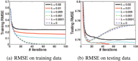
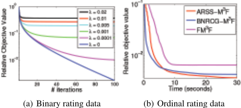
In this section, to demonstrate the sensitivity of regularization, we perform experiments on the small-scale binary matrix. To illustrate the impact of the regularization in the proposed methods, we test BNRCG-M3F with various regularization parameters λ. Figure 1 reports the training RMSE and testing RMSE. The convergence is shown in Figure 2(a). As can be seen, the regularization is crucial for preventing overfitting.
Convergence of M3F on Ordinal Rating Data
In this section, we perform experiments on the small-scale ordinal matrix. We compare the proposed algorithms with the six baseline methods and collect the convergence behavior of the three M3F methods. The ground-truth rank is used as the estimated rank for all methods excluding ARSS-M3F.
The convergence behavior of our methods and FM3F is illustrated in Figure 2(b), which shows that our methods can converge better and faster. Table 2 reports the resultant RMSE on the testing set and the computational time of each method on the small-scale synthetic ordinal rating data set.
Scalability of M3F on Ordinal Rating Data
In this section, we perform experiments on the large-scale ordinal matrix. We compare our methods with the 5 baseline algorithms. We use the ground-truth rank as the estimated rank for all methods except ARSS-M3F. The average estimated rank of ARSS-M3F is 42, which is close to the groundtruth rank of 50. According to the estimated rank in the two synthetic datasets, the latent factor detection of ARSS-M3 is effective. The RMSE on the testing set and computational time of each algorithm are listed in Table 2.
| Table 1: Statistics of the Real-world Data Sets. | |||
|---|---|---|---|
| Data Sets | # users | # items | # ratings |
| Movielens 1M | 6,040 | 3,952 | 1,000,209 |
| Movielens 10M | 71,567 | 10,681 | 10,000,054 |
| Netflix | 480,189 | 17,770 | 100,480,507 |
| Yahoo! Music Track 1 | 1,000,990 | 624,961 | 262,810,175 |
4.2 Real-world Experiments
In real-world data experiments, to demonstrate the significance of the hinge loss to the rating data and effectiveness of latent factor estimation of our method, we study four realworld large scale data sets, namely Movielens 1M, Movielens 10M data set, Netflix data set and Yahoo! Music Track 1 data set. The baseline methods include FM3F, GROUSE, LMAFIT, ScGrassMC, LRGeomCG and RTRMC.
Table 1 lists the size statistics of the four data sets. The vast majority (99.71%) of ratings in Yahoo! Music Track 1 are multiples of ten. For convenience, we only consider these ratings. For Movielen 10M and Yahoo! Music Track 1, we map the ratings to ordinal integer values before the experiment. For each data set, we sample 80% of data into the training set and the rest into the testing set.
Table 2 reports the computational time of all comparison methods and testing RMSE on the four data sets. According to the resultant RMSE, compared to other loss measure, i.e. least square loss, our method can recover the matrix with lower error. Note that in all experiments in both synthetic and real-world data, no model selection cost is included for all comparison methods. If model selections are considered, the comparison methods will cost much more time. Some results for GROUSE and M3F are not available due to their high computation cost. From the table, ARSS-M3F and BNRCG-M3F recover the rating matrix efficiently and outperform other comparison methods in terms of RMSE on the four real-world data sets. It is worth mentioning that though LRGeomCG shows faster speed on Yahoo data set, it achieves much worse RMSE than M3F based methods.
5 Conclusion
To deal with the ordinal discrete ratings in recommendation systems, M3F is proposed. However, existing M3F methods is faced with the scalability and latent factor detection issues. To address the two challenges, we present ARSSM3F, a scalable M3F method based on active Riemannian subspace search. Specifically, the proposed algorithm first treat the M3F problem as the fixed number of latent factors and solve it using BNRCG. In the meantime, a simple and efficient active subspace search approach is applied to automatically compute the number of latent factors. Experiments on both synthetic and real-world data demonstrate that the proposed method can provide competitive performance.
| Methods | Small Synthetic* | Large Synthetic* | Movielens 1M† | Movielens 10M† | Netflix† | Yahoo Music† | ||||||
|---|---|---|---|---|---|---|---|---|---|---|---|---|
| RMSE | Time | RMSE | Time | RMSE | Time | RMSE | Time | RMSE | Time | RMSE | Time | |
| FM3 F [Rennie and Srebro, 2005] | 0.3811 | 11.99 | 0.3899 | 2186 | 0.9344 | 212.2051 | 0.9143 | 13001 | 1.0971 | 65662 | - | - |
| GROUSE [Balzano et al., 2010] | 0.4718 | 27.84 | 0.512 | 11214 | 0.9225 | 39.4184 | 0.8653 | 3853 | - | - | - | - |
| LMAFIT [Wen et al., 2012] | 0.4701 | 6.08 | 0.4973 | 827 | 0.9373 | 19.9465 | 0.8424 | 832 | 0.9221 | 4374 | 24.222 | 24349 |
| ScGrassMC [Ngo and Saad, 2012] | 0.4638 | 10.19 | 0.4714 | 2149 | 0.9372 | 21.3109 | 0.8427 | 917 | 0.9192 | 5787 | 24.7982 | 37705 |
| LRGeomCG [Vandereycken, 2013] | 0.4679 | 6.01 | 0.4904 | 814 | 0.9321 | 10.2484 | 0.849 | 312 | 0.9015 | 3151 | 25.2279 | 8666 |
| RTRMC [Boumal and Absil, 2011] | 0.4676 | 8.68 | 0.4715 | 884 | 0.9311 | 14.1038 | 0.846 | 673 | 0.9102 | 6465 | 24.5971 | 32592 |
| BNRCG-M3 F | 0.3698 | 5.34 | 0.3915 | 635 | 0.9285 | 13.4437 | 0.8437 | 714 | 0.9022 | 4118 | 23.8573 | 24631 |
| ARSS-M3 F | 0.3693 | 5.33 | 0.3684 | 542 | 0.9222 | 9.5482 | 0.8411 | 650 | 0.9001 | 3583 | 23.7902 | 22065 |
Acknowledgement
This work was in part supported by the 973 Program (2015CB352300), in part supported by the Australian Research Council Future Fellowship FT130100746, the Data to Decisions Cooperative Research Centre, Australia, and the ARC Grant DP140102270 and DE130101311.
A Appendix A: Computation of gradf(X, θ)
According to [Vandereycken, 2013], a tangent vector η ∈ TMr is represented as η = UMVT+UpVT+UVT p (see equation (7) for details). By definition, the Riemannian gradient of f(X, θ) w.r.t. X, denoted by gradf(X, θ), at X = Udiag(σ)VT can be calculated by PTXMr (G), where PTXMr (Z) = PUZPV + P ⊥ U ZPV +PUZP ⊥ V is the projection of G onto the tangent space T Mr. Let Ξ = λdiag(σ - ν/σ3 ). For convenience, we first present the computation of gradf(X, θ) in Algorithm 3.
Lemma 1. Suppose Up, Vp, and M are obtained from Algorithm 3, then gradf (X, θ) = UMVT + UpVT + UVT p .
Algorithm 3 Compute Riemannian gradient gradf (X).
- 1: Let Ξ = λdiag(σ - ν/σ3 ), and compute ̂G via (9).
- 2: Compute Gu = ̂GTU, and Gv = ̂GV.
- 3: Compute ̂M = UTGv .
- 4: Compute Up = Gv - ÛM, and Vp = Gu - V̂MT .
- 6: Update M = ̂M + Ξ.
- 6: Output Up, Vp, and M, and gradf(X, θ) = UMVT+ UpVT+UVT p .
Proof. To verify the validity of Algorithm 3, we just need to show that, PTXMr (G) = UMVT+UpVT+UVT p .
Notice that, UTU = I and VTV = I. On one hand, we have PTXMr (G) = PTXMr ( ̂G + UΞVT) = ̂GPV + PU ̂G - PU ̂GPV + UΞVT. On the other hand, according to Algorithm 3, we have η = UMVT+UpVT+UVT p = ÛMVT + UpVT+UVT p +UΞVT = ̂GVVT +UUT ̂GÛMVT + UΞVT , which actually equals to PTXMr (G). This completes the proof.
B Appendix B: Proof of Proposition 1
The proof parallels the proof in [Vandereycken, 2013]. Notice that, the optimization on θ is conducted in Euclidian space RL-1 . Moreover, {θt} is bounded; otherwise ℓ(X, θ) will go to infinity according to (4). Without loss of generality, suppose θt ∈ [-l, l]L-1 , where l > 0 is a finite number. Following [Vandereycken, 2013], we can also show that {Xt} stay in a closed and bounded subset of Mr.
Let Ψ = {X ∈ Mr, f(X, θ) ≤ f(X0, θ0)} be the level set at (X0, θ0). Due to the line search, we have ℓ(Xt, θt) + λ2 (||Xt||2F + ν||X†t ||2F ) ≤ f(X0, θ0). Therefore, we have λ2 ||Xt||2F ≤ f(X0, θ0), which implies σ1 = √||Xt||2F ≤ √2f(X0, θ0)/λ. Here, σ1 denotes the largest singular value of Xt. Similarly, we have νλ 2 ||X†t ||2F = ∑ri=1 νλ 2σ2 i ≤ f(X0, θ0), which implies that νλ 2σ2 i ≤ f(X0, θ0), ∀i ∈ {1, ..., r}. This further implies that σr ≥ √νλ/2f(X0, θ0), where σr is the least singular value of Xt.
Clearly, all Xt stay inside the set S = {X ∈ Mr : σ1 ≤ √2f(X0, θ0)/λ, σr ≥ √νλ/2f(X0, θ0)}, which is closed and bounded, hence compact.
Now we complete the proof by contradiction. Without loss of generality, suppose limt→∞ ||gradf(Xt, θt)||F + ||∇θt f(Xt, θt)||2 ̸= 0, then there exists an ϵ > 0, and a subsequence in {(Xt, θt)}t∈Γ such that ||gradf(Xt, θt)||F + ||∇θf(Xt, θt)||2 ≥ ϵ > 0 for all t ∈ Γ. Since Xt ∈ S and θt is constrained in [-l, l]L-1 , the subsequence {(Xt, θt)}t∈Γ should have a limit point (X∗ , θ∗ ) in S × [-l, l]L-1 . By continuity of gradf(X, θ) and ∇θf(X, θ) (which can be easily verified for squared hinge loss), this implies that ||gradf(Xt, θt)||F ≥ ϵ which contradicts Theorem 4.3.1 in [Absil et al., 2008] that every accumulation point is a critical point of f(X, θ). We therefore conclude that limt→∞ ||gradf(Xt, θt)||F = 0 and limt→∞ ||∇θf (Xt, θt)||2 = 0.
@inproceedings{ijcai2015p560,
  title     = {Scalable Maximum Margin Matrix Factorization by Active Riemannian Subspace Search},
  author    = {Yan, Yan and Tan, Mingkui and Tsang, Ivor W. and Yang, Yi and Zhang, Chengqi and Shi, Qinfeng},
  booktitle = {Proceedings of the Twenty-Fourth International Joint Conference on
               Artificial Intelligence, {IJCAI-15}},
  publisher = {International Joint Conferences on Artificial Intelligence},
  editor    = {Qiang Yang and Michael Wooldridge},
  pages     = {3988--3993},
  year      = {2015},
  month     = {7},
  note      = {Special Track on Machine Learning},
  url       = {https://ijcai.org/proceedings/2015/560},
}
TY - CPAPER TI - Scalable Maximum Margin Matrix Factorization by Active Riemannian Subspace Search AU - Yan, Yan AU - Tan, Mingkui AU - Tsang, Ivor W. AU - Yang, Yi AU - Zhang, Chengqi AU - Shi, Qinfeng T2 - Proceedings of the Twenty-Fourth International Joint Conference on Artificial Intelligence, IJCAI-15 PB - International Joint Conferences on Artificial Intelligence PY - 2015 SP - 3988 EP - 3993 UR - https://ijcai.org/proceedings/2015/560 ER -Copied
Machine-readable versions of this paper, for tools and AI agents:





